Kernel Fisher Discriminant Analysis#
Provided by
Motahare Namakin Contact : Motahare.namakin@gmail.com
Farkhondeh Arazi Contact : farkhondeh.arzi@gmail.com

KFDA is an extension of Fisher Discriminant Analysis (FDA) that works in a high-dimensional feature space induced by a kernel function. It is particularly useful for non-linear classification problems where the linear decision boundary of FDA is insufficient.
Two classes#
To extend LDA to non-linear mappings, the data, given as the \(n\) points \(x_i\), can be mapped to a new feature space, 𝐹, via some function \(\phi\). In this new feature space, the function that needs to be maximized is:
\(J(w)=\frac{w^{T}S^{\phi}_{B}w}{w^{T}S^{\phi}_{w}w}\)
where
\(S^{\phi}_{B}=(m^{\phi}_{2}-m^{\phi}_{1})(m^{\phi}_{2}-m^{\phi}_{1})^{T}\)
\(S^{\phi}_{w}=\Sigma^\phi_1+\Sigma^\phi_2=\sum\limits_{i=1,2}^{}\sum\limits_{j=1}^{n_{i}}(\phi(x_j^i)-m_i^\phi)(\phi(x_j^i)-m_i^\phi)^T\)
\(S^{\phi}_{w}=\sum\limits_{1}^{\phi}+\sum\limits_{2}^{\phi}=\sum\limits_{i=1,2}^{}\sum\limits_{j=1}^{n_{i}}(\phi(x_j^i)-m_i^\phi)(\phi(x_j^i)-m_i^\phi)^T\)
In addition, \(m_i^\phi\), which is the mean of the data points of class 𝑖 in the \(\phi-\mathrm{space}\), is defined as follows:
\(m_i^\phi=\frac{1}{n_{i}}\sum\limits_{j=1}^{n_{i}}\phi(x^i_j)\)
Where \(x_j^i\) is the 𝑗-th data point from class 𝑖.
Further, note that 𝑤 ∈ 𝐹. Explicitly computing the mappings 𝜙(𝑥𝑖) and then performing LDA can be computationally expensive, and in many cases intractable. For example, 𝐹 may be infinitely dimensional. Thus, rather than explicitly mapping the data to 𝐹, the data can be implicitly embedded by rewriting the algorithm in terms of dot products and using kernel functions in which the dot product in the new feature space is replaced by a kernel function, 𝑘(𝑥,𝑦)=𝜙(𝑥)⋅𝜙(𝑦).
LDA can be reformulated in terms of dot products by first noting that 𝑤 will have an expansion of the form:
\(w=\sum\limits_{i=1}^{n}\alpha_{i}\phi(x_i)\)
Then note that
\(w^tm_i^\phi=\frac{1}{n_i}\Sigma^{n}_{j=1}\Sigma^{n_i}_{k=1}\alpha_{j}\phi^T(x_i)\phi(x_k^i)=\frac{1}{n_i}\Sigma^{n}_{j=1}\Sigma^{n_i}_{k=1}\alpha_{j}k(x_j,x_k^i)=\alpha^TM_i\)
\(w^tm_i^\phi=\frac{1}{n_i}\sum\limits_{j=1}^{n}\sum\limits_{k=1}^{n_i}\alpha_{j}\phi^T(x_i)\phi(x_k^i)=\frac{1}{n_i}\sum\limits_{j=1}^{n}\sum\limits_{k=1}^{n_i}\alpha_{j}k(x_j,x_k^i)=\alpha^TM_i\)
where
\((M_i)j=\frac{1}{n_{i}}\Sigma^{n_i}_{k=1}k(x_j,x_k^i)\)
\((M_i)j=\frac{1}{n_{i}}\sum\limits_{k=1}^{n_i}k(x_j,x_k^i)\)
The numerator of 𝐽(𝑤) can then be written as:
\(w^TS^\phi_Bw=w^T(m^{\phi}_{2}-m^{\phi}_{1})(m^{\phi}_{2}-m^{\phi}_{1})^{T}w\)
Considering that \((m^{\phi}_{2}-m^{\phi}_{1})^Tw=(w^T(m^{\phi}_{2}-m^{\phi}_{1}))^{T}\) , we only need to find the specified part:
\(w^T(m^{\phi}_{2}-m^{\phi}_{1})=\alpha^TM_2-\alpha^TM_1=\alpha^T(M_2-M_1)\to \\ w^TS^\phi_Bw=\alpha^T(M_2-M_1)(M_2-M_1)^T\alpha=\alpha^TM\alpha \\ M=(M_2-M_1)(M_2-M_1)^T\)
And for the denominator of the expression 𝐽(𝑤), we have: \(w^TS^\phi_ww=\left(\sum\limits_{i=1}^{n}\alpha_i\phi^T(x_i)\right)\left(\sum\limits_{i=1,2}^{}\sum\limits_{j=1}^{n_i}(\phi(x_j^i)-m_i^\phi)(\phi(x_j^i)-m_i^\phi)^T\right)\left(\sum\limits_{i=1}^{n}\alpha_i\phi(x_i)\right)\\ =\sum\limits_{j=1,2}^{}\sum\limits_{i=1}^{n}\sum\limits_{l=1}^{n_j}\sum\limits_{k=1}^{n}(\alpha_i\phi^T(x_i)(\phi(x_j^i)-m_i^\phi)(\phi(x_j^i)-m_i^\phi)^T)\alpha_i\phi(x_i))\\ =\sum\limits_{j=1,2}^{}\sum\limits_{i=1}^{n}\sum\limits_{l=1}^{n_j}\sum\limits_{k=1}^{n}\left(\alpha_ik(x_i,x_l^j)-\frac{1}{n_i}\sum\limits_{p=1}^{n_i}\alpha_ik(x_j,x_p^i)\right)\left(\alpha_ik(x_l,x_k^j)-\frac{1}{n_i}\sum\limits_{q=1}^{n_i}\alpha_kk(x_q,x_k^i)\right)\\ =\sum\limits_{j=1,2}^{}\left[ \sum\limits_{i=1}^{n}\sum\limits_{l=1}^{n_j}\sum\limits_{k=1}^{n}\left( \alpha_i\alpha_kk(x_i,x_l^j)k(x_k,x_l^j)-\frac{\alpha_i\alpha_k}{n_i}\sum\limits_{p=1}^{n_i}k(x_i,x_l^i)k(x_k,x_p^i) \right) \right]\\ =\sum\limits_{j=1,2}^{}\alpha^T\left( K_jK_j^T-K_j1_{n_j}K_j^T \right)\alpha\\ =\alpha^T\left[ \sum\limits_{j=1,2}^{}\left( K_jK_j^T-K_j1_{n_j}K_j^T \right) \right]\alpha=\alpha^TN\alpha\\ N=\left[ \sum\limits_{j=1,2}^{}\left( K_jK_j^T-K_j1_{n_j}K_j^T \right) \right]\)
\(J(\alpha)=\frac{\alpha^TM\alpha}{\alpha^TN\alpha}\)
\(I\) is the identity matrix, and \(1_{n_j}\) the matrix with all entries equal to 1/\(n_𝑗\). This identity can be derived by starting out with the expression for \(w^TS^\phi_ww\) and using the expansion of 𝑤 and the definitions of \(S^\phi_w\) and \(m^\phi_i\)
We take the derivative with respect to 𝛼:
\(\frac{d\;J(\alpha)}{d\;\alpha}=0\to (\alpha^TM\alpha)N\alpha-(\alpha^TN\alpha)M\alpha=0\to (\alpha^TM\alpha)N\alpha=(\alpha^TN\alpha)M\alpha\)
In the above equation, the highlighted parts are scalars. Therefore, since only the direction of 𝑤 and consequently the direction of 𝛼 is important to us, we can ignore them.
\(\to N\alpha=M\alpha\to \alpha=N^{-1}M\alpha=N^{-1}(M_2-M_1)(M_2-M_1)^T\alpha\\ \alpha=N^{-1}(M_2-M_1)\)
Therefore, to find the label of each x, we do the following:
\(y(x)=w^T\phi(x)=\sum\limits_{i=1}^{n}a_ik(x_i,x)\)
\(label=f(x)=^{argmin}_{\;\;\;j}D(y(x),\bar{y}_j)\)
where \(\bar{y}_j\) is the average projected data for class \(j\). And \(D(.,.)\) is a distance function.
from sklearn.metrics import accuracy_score

def accuracy(model, x, y):
  predicted = model.predict(x)
  accuracy = accuracy_score(y, predicted)
  print("Accuracy:", accuracy)
import matplotlib.pyplot as plt
from sklearn.datasets import make_moons

def generate_two_moons():
  # Generate two moons data
  X, y = make_moons(n_samples=1000, noise=0.1, random_state=42)

  # Plot the data
  plt.figure(figsize=(8, 6))
  plt.scatter(X[y == 0][:, 0], X[y == 0][:, 1], color='red', label='Class 0')
  plt.scatter(X[y == 1][:, 0], X[y == 1][:, 1], color='blue', label='Class 1')
  plt.xlabel('Feature 1')
  plt.ylabel('Feature 2')
  plt.title('Two Moons Data')
  plt.legend()
  plt.show()

  return X, y
import numpy as np
import matplotlib.pyplot as plt
from sklearn.datasets import make_moons
from sklearn.model_selection import train_test_split

def create_moon(center, rotation, n_samples=1000, noise=0.1):
    X, y = make_moons(n_samples=n_samples, noise=noise)
    # Apply rotation
    theta = np.deg2rad(rotation)
    rotation_matrix = np.array([[np.cos(theta), -np.sin(theta)], [np.sin(theta), np.cos(theta)]])
    X = X.dot(rotation_matrix)
    # Apply translation
    X += center
    return X, y

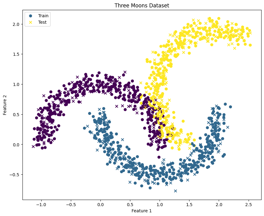
def generate_three_moons():
  # Generate three moons datasets
  X1, y1 = create_moon(center=[0, 0], rotation=0, n_samples=1000, noise=0.1)
  X2, y2 = create_moon(center=[2, 2], rotation=120, n_samples=1000, noise=0.1)

  X2 = X2[y2 != 0]
  y2 = y2[y2 != 0]

  # Combine datasets
  X = np.vstack([X1, X2])
  y = np.hstack([y1, y2 + 2])

  # Split the combined dataset into training and testing sets
  X_train, X_test, y_train, y_test = train_test_split(X, y, test_size=0.3, random_state=42)

  # Plot the combined dataset
  plt.figure(figsize=(10, 8))
  plt.scatter(X_train[:, 0], X_train[:, 1], c=y_train, cmap='viridis', marker='o', label='Train')
  plt.scatter(X_test[:, 0], X_test[:, 1], c=y_test, cmap='viridis', marker='x', label='Test')
  plt.xlabel('Feature 1')
  plt.ylabel('Feature 2')
  plt.title('Three Moons Dataset')
  plt.legend()
  plt.show()

  return X, y
import numpy as np
import matplotlib.pyplot as plt
from sklearn.datasets import make_moons
from sklearn.discriminant_analysis import LinearDiscriminantAnalysis
from sklearn.preprocessing import StandardScaler

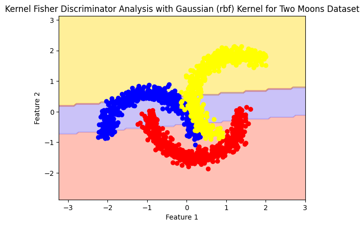
def plot_boundry_decision(model, X, y):
  # Scale the features
  scaler = StandardScaler()
  X_scaled = scaler.fit_transform(X)

  # # Plot the decision boundary
  x_min, x_max = X_scaled[:, 0].min() - 1, X_scaled[:, 0].max() + 1
  y_min, y_max = X_scaled[:, 1].min() - 1, X_scaled[:, 1].max() + 1
  xx, yy = np.meshgrid(np.linspace(x_min, x_max, 100), np.linspace(y_min, y_max, 100))
  model.fit(X_scaled, y)

  # Plot the decision boundary
  Z = model.predict(np.c_[xx.ravel(), yy.ravel()])
  Z = Z.reshape(xx.shape)

  plt.contourf(xx, yy, Z, alpha=0.4, colors=['mediumslateblue', 'mediumslateblue', 'tomato', 'gold'])

  color = []
  for i in range(len(y)):
    if y[i] == 0:
        color.append('blue')
    elif y[i] == 1:
      color.append('red')
    elif y[i] == 3:
      color.append('yellow')
  plt.scatter(X_scaled[:, 0], X_scaled[:, 1], c=color)
  plt.xlabel('Feature 1')
  plt.ylabel('Feature 2')
  plt.title('Kernel Fisher Discriminator Analysis with Gaussian (rbf) Kernel for Two Moons Dataset')
  plt.show()
Create Module kfda#
The following lines define the class Kfda, which inherits from three mixins BaseEstimator, ClassifierMixin, and TransformerMixin from the scikit-learn library. These three mixins provide basic methods and attributes for a machine learning estimator.
The init function sets initial values for the class.
n_components specifies the number of Fisher directions onto which the data are projected.
Kernel specifies the type of kernel used for computing the kernel matrix.
robustness_offset adds a small value to the diagonal of the matrix to prevent numerical issues (matrix becoming singular).
The classes are defined as: $\( \mathrm{classes} \ i=\left\{ y_i \ ;\ y_i \in y \right\} \)$
The one-hot encoding of the labels ( y ) is defined as:
The kernel matrix ( K ) is defined as: $\(K=\kappa(X,X)\)$
The mean embedding of the ( i )-th class ( M_i ) is defined as: $\((M_i)=\frac{1}{n_i}\sum\limits_{k=1}^{n_i}k(x_j,x^i_k)\)$
leading to the class mean matrix ( M_{\mathrm{class}} ): $\(M_{\mathrm{class}}=Y_{\mathrm{onehot}}^TK/\sum_{}^{}(Y_{\mathrm{onehot}})\)$
The matrix ( N ) is defined as: $\(N=K\left( K-M_{\mathrm{class}}\left[ Y_{\mathrm{onehot}} \right] \right)\)$
The adjusted matrix ( N ) is given by: $\(N=N+\epsilon I\)$
The difference between the mean embedding of the ( i )-th class and the overall mean is given by:
The outer product of the difference between the mean embedding of the ( i )-th class and the overall mean is given by: $\(\left( M_i-M_* \right)\left( M_i-M_* \right)^T\)$
The matrix equation is given by: $\(MA=\lambda NA\)$
The center of every class can be found by: $\(\mathrm{centroids}=M_{\mathrm{class}}w\)$
"""Module kfda"""
import warnings
from scipy.sparse.linalg import eigsh
from scipy.sparse import eye
from sklearn.base import BaseEstimator, ClassifierMixin, TransformerMixin
from sklearn.metrics import pairwise_kernels
from sklearn.neighbors import NearestCentroid
from sklearn.utils.multiclass import unique_labels
from sklearn.preprocessing import OneHotEncoder
import numpy as np


class Kfda(BaseEstimator, ClassifierMixin, TransformerMixin):

    def __init__(self, n_components=2, kernel='linear', robustness_offset=1e-8,
                 **kwds):
        self.kernel = kernel
        self.n_components = n_components
        self.kwds = kwds
        self.robustness_offset = robustness_offset

        if kernel is None:
            self.kernel = 'linear'

    def fit(self, X, y):
        # 1.
        self.classes_ = unique_labels(y)
        if self.n_components > self.classes_.size - 1:
            warnings.warn(
                "n_components > classes_.size - 1."
                "Only the first classes_.size - 1 components will be valid."
            )
        self.X_ = X
        self.y_ = y

        # 2.
        y_onehot = OneHotEncoder().fit_transform(
            self.y_[:, np.newaxis])

        # 3.
        K = pairwise_kernels(
            X, X, metric=self.kernel, **self.kwds)

        m_classes = y_onehot.T @ K / y_onehot.T.sum(1)

        # 4.
        indices = (y_onehot @ np.arange(self.classes_.size)).astype('i')
        # 5.
        N = K @ (K - m_classes[indices])

        # Add value to diagonal for rank robustness
        # 6.
        N += eye(self.y_.size) * self.robustness_offset

        # 7.
        m_classes_centered = m_classes - K.mean(1)
        # 8.
        M = m_classes_centered.T @ m_classes_centered

        # Find weights
        # 9.
        w, self.weights_ = eigsh(M, self.n_components, N, which='LM')
        # self.weights_ = solve_ma_eq_na_iterative(M, N)

        # Compute centers
        # 10.
        centroids_ = m_classes @ self.weights_
        centroids_ = np.asarray(centroids_)

        # Train nearest centroid classifier
        self.clf_ = NearestCentroid().fit(centroids_, self.classes_)

        return self

    def transform(self, X):
        """Project the points in X onto the fisher directions.

        Parameters
        ----------
        X : {array-like} of shape (n_samples, n_features) to be
            projected onto the fisher directions.
        """
        return pairwise_kernels(
            X, self.X_, metric=self.kernel, **self.kwds
        ) @ self.weights_

    def predict(self, X):

        projected_points = self.transform(X)
        predictions = self.clf_.predict(projected_points)

        return predictions

    def fit_additional(self, X, y):

        new_classes = np.unique(y)

        projections = self.transform(X)
        y_onehot = OneHotEncoder().fit_transform(
            y[:, np.newaxis])
        new_centroids = y_onehot.T @ projections / y_onehot.T.sum(1)

        concatenated_classes = np.concatenate([self.classes_, new_classes])
        concatenated_centroids = np.concatenate(
            [self.clf_.centroids_, new_centroids])

        self.clf_.fit(concatenated_centroids, concatenated_classes)

        return self
import matplotlib.pyplot as plt
from sklearn.datasets import make_moons
from sklearn.model_selection import train_test_split
import numpy as np

# Generate the two moons dataset
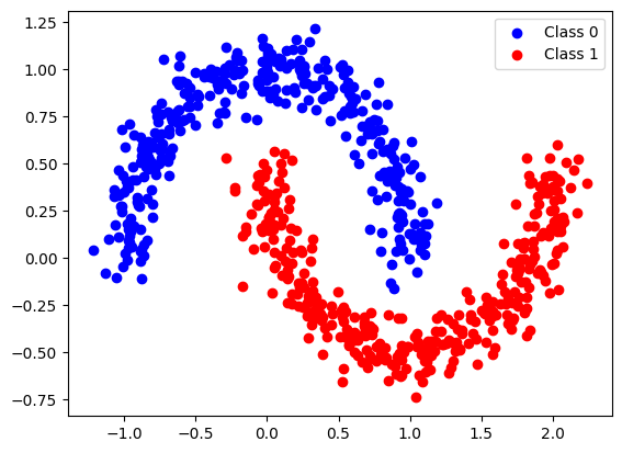
X, y = make_moons(n_samples=1000, noise=0.1, random_state=42)

# Split the data into training and testing sets
X_train, X_test, y_train, y_test = train_test_split(X, y, test_size=0.3, random_state=42)

# Plot the training data
plt.scatter(X_train[y_train == 0][:, 0], X_train[y_train == 0][:, 1], color='blue', label='Class 0')
plt.scatter(X_train[y_train == 1][:, 0], X_train[y_train == 1][:, 1], color='red', label='Class 1')
plt.legend()
plt.show()
Linear#
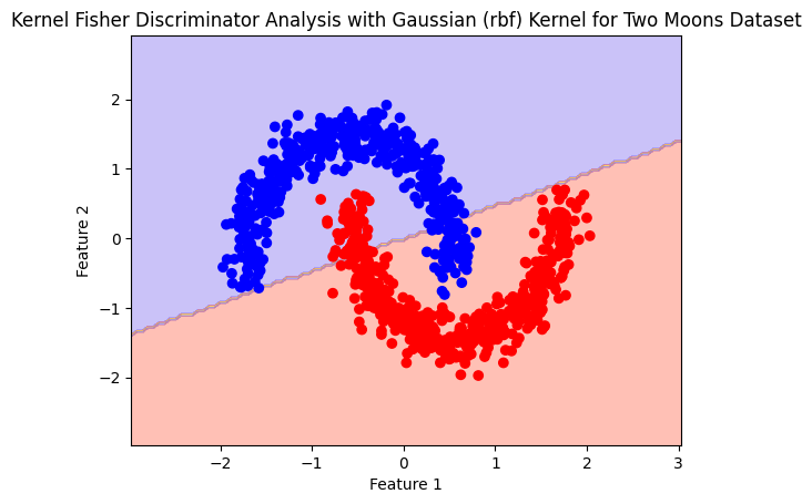
model= Kfda(kernel='linear', n_components = 1)
model.fit(X,y)
Kfda(n_components=1)In a Jupyter environment, please rerun this cell to show the HTML representation or trust the notebook.
On GitHub, the HTML representation is unable to render, please try loading this page with nbviewer.org.
Kfda(n_components=1)
from sklearn.metrics import accuracy_score
# Assuming you have already fit the model as follows:
# model = Kfda(kernel='linear', n_components=1)
# model.fit(X, y)

# Predict the labels on the same dataset
y_pred = model.predict(X)

# Calculate and print accuracy
acc = accuracy_score(y, y_pred)
print(f"Accuracy: {acc}")
Accuracy: 0.877
plot_boundry_decision(model, X, y)
polynomial#
polynomial_model= Kfda(kernel='polynomial')
polynomial_model.fit(X,y)
C:\Users\Hadi\AppData\Local\Temp\ipykernel_4304\3548760067.py:29: UserWarning: n_components > classes_.size - 1.Only the first classes_.size - 1 components will be valid.
  warnings.warn(
Kfda(kernel='polynomial')In a Jupyter environment, please rerun this cell to show the HTML representation or trust the notebook.
On GitHub, the HTML representation is unable to render, please try loading this page with nbviewer.org.
Kfda(kernel='polynomial')
from sklearn.metrics import accuracy_score
# Assuming you have already fit the model as follows:
# model = Kfda(kernel='linear', n_components=1)
# model.fit(X, y)

# Predict the labels on the same dataset
y_pred = model.predict(X)

# Calculate and print accuracy
acc = accuracy_score(y, y_pred)
print(f"Accuracy: {acc}")
Accuracy: 0.859
plot_boundry_decision(polynomial_model, X, y)
C:\Users\Hadi\AppData\Local\Temp\ipykernel_4304\3548760067.py:29: UserWarning: n_components > classes_.size - 1.Only the first classes_.size - 1 components will be valid.
  warnings.warn(
RBF#
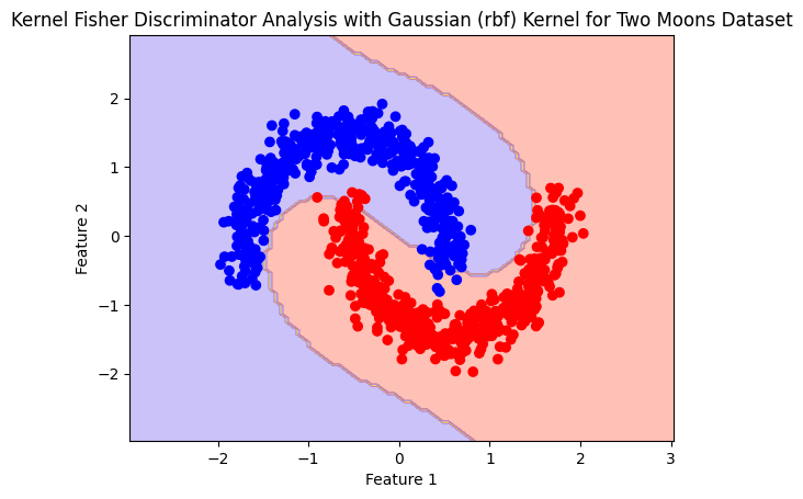
rbf_model= Kfda(kernel='rbf')
rbf_model.fit(X,y)
C:\Users\Hadi\AppData\Local\Temp\ipykernel_4304\3548760067.py:29: UserWarning: n_components > classes_.size - 1.Only the first classes_.size - 1 components will be valid.
  warnings.warn(
Kfda(kernel='rbf')In a Jupyter environment, please rerun this cell to show the HTML representation or trust the notebook.
On GitHub, the HTML representation is unable to render, please try loading this page with nbviewer.org.
Kfda(kernel='rbf')
from sklearn.metrics import accuracy_score
# Assuming you have already fit the model as follows:
# model = Kfda(kernel='linear', n_components=1)
# model.fit(X, y)

# Predict the labels on the same dataset
y_pred = model.predict(X)

# Calculate and print accuracy
acc = accuracy_score(y, y_pred)
print(f"Accuracy: {acc}")
Accuracy: 0.859
plot_boundry_decision(rbf_model, X, y)
C:\Users\Hadi\AppData\Local\Temp\ipykernel_4304\3548760067.py:29: UserWarning: n_components > classes_.size - 1.Only the first classes_.size - 1 components will be valid.
  warnings.warn(

Multi classes#
Using the determinant for scalirization the objective function
The extension to cases where there are more than two classes is relatively straightforward.Let 𝑐 be the number of classes. Then multi-class KFD involves projecting the data into a (𝑐−1)-dimensional space using (𝑐−1) discriminant functions
\(y_i=w_i\phi(x),i=1,\cdots,C-1\)
This can be written in matrix notation
\(Y=W^T\phi(x)\)
where the 𝑤𝑖 are the columns of 𝑊. Further, the between-class covariance matrix is now
\(S^\phi_B=\Sigma^C_{i=1}n_i(m_i^\phi-m^\phi)(m_i^\phi-m^\phi)^T\)
\(S^\phi_B=\sum\limits_{i=1}^{C}n_i(m_i^\phi-m^\phi)(m_i^\phi-m^\phi)^T\)
where \(m^\phi\) is the mean of all the data in the new feature space. The within-class covariance matrix is
The solution is now obtained by maximizing
\(J(W)=\frac{\left| W^TS^\phi_BW \right|}{\left| W^TS^\phi_wW \right|}\to\)\(J(A)=\frac{\left| A^TMA \right|}{\left| A^TNA \right|}\)
The kernel trick can again be used and the goal of multi-class KFD becomes
\(A^*=^{argmax}_{\;\;\;A}J(A)\)
where \(A=\left\{ \alpha_1,\alpha_2,\cdots,\alpha_{c-1} \right\}\) and
\(M=\Sigma^C_{i=1}n_i(M_i-M_*)(M_i-M_*)^T , N=\Sigma^C_{i=1}K_i(I-1_{n_i})K^T_i\)
\(M=\sum_\limits{i=1}^{C}n_i(M_i-M_*)(M_i-M_*)^T , N=\sum_\limits{i=1}^{C}K_i(I-1_{n_i})K^T_i\)
We want to calculate \(\frac{d J(A)}{dA}=0\)
\(J(A)=\frac{\mathrm{det}(A^TMA)}{\mathrm{det}(A^TNA)}\)
To calculate the derivative of the determinant, we have:
\(d(\mathrm{det}(X))=\mathrm{det}(X)\cdot trace(X^{-1}dX)\)
Therefore, to find the relationship: \(\frac{d}{dA}\left( \frac{\mathrm{det}(A^TMA)}{\mathrm{det}(A^TNA)} \right)\)
By changing the variables \(u=\mathrm{det}(A^TMA)\) and \(v=\mathrm{det}(A^TNA)\), the expression of J transforms to:
\(J(A)=\frac{u}{v}\to \frac{dJ}{dA}=\frac{v\frac{du}{dA}-u\frac{dv}{dA}}{v^2}\)
The derivative of 𝑢 with respect to 𝐴 is:
\(du=\mathrm{det}(A^TMA)\cdot trace\left( (A^TMA)^{-1}d(A^TMA) \right)\)
And since:
\(\frac{d}{dA}(A^TMA)=MA+A^TM\)
We have:
\(\frac{du}{dA}=\mathrm{det}(A^TMA)\cdot trace\left( (A^TMA)^{-1} (MA+A^TM)\right)\)
And similarly for \(v=\mathrm{det}(A^TNA)\) we have:
\(\frac{dv}{dA}=\mathrm{det}(A^TNA)\cdot trace\left( (A^TNA)^{-1} (NA+A^TN)\right)\)
and:
\(\frac{dJ}{dA}=\frac{\mathrm{det}(A^TMA)\cdot trace\left( (A^TMA)^{-1} (MA+A^TM)\right)-\mathrm{det}(A^TNA)\cdot trace\left( (A^TNA)^{-1} (NA+A^TN)\right)}{d(A^TNA)^2}\)
in order for \(\frac{dJ}{dA}=0\), we must set its numerator equal to zero:
\(\mathrm{det}(A^TMA)\cdot trace\left( (A^TMA)^{-1} (MA+A^TM)\right)=\mathrm{det}(A^TNA)\cdot trace\left( (A^TNA)^{-1} (NA+A^TN)\right)\)
And we assume that A is chosen in a way that its determinant does not become zero.
\(trace\left( (A^TMA)^{-1} (MA+A^TM)\right)=trace\left( (A^TNA)^{-1} (NA+A^TN)\right)\)
Therefore, we have:
\(MA=\lambda NA,\lambda =\frac{\mathrm{det}(A^TMA)}{\mathrm{det}(A^TNA)}\)
Therefore, the optimal \(A^*\) can be found by either finding the eigenvector corresponding to the first \(c-1\) eigenvalue of \(N^{-1}M\) or solving the equation \(MA=\lambda NA\).
Replacing the determinant with the trace in the cost function:
Now, if we use the trace instead of the determinant in the function J to convert the relation to a scalar we will have:
\(J(A)=\frac{trace(A^TMA)}{trace(A^TNA)}\)
By changing the variables \(u=trace(A^TMA)\) and \(v=trace(A^TNA)\),we have:
\(J(A)=\frac{u}{v}\to \frac{dJ}{dA}=\frac{v\frac{du}{dA}-u\frac{dv}{dA}}{v^2}\)
To calculate the derivative of trace, we have:
\(d\left( trace(X) \right)=trace\left( d(X) \right)\)
Therefore, for du and dv, we have:
\(du=2\cdot trace(MAdA^T)\)
\(dv=2\cdot trace(NAdA^T)\)
So, the expression for \(\frac{dJ}{dA}\) can be rewritten as:
\(\frac{dJ}{dA}=\frac{trace(A^TNA)\cdot 2\cdot trace(MAdA^T)-trace(A^TMA)\cdot 2\cdot trace(NAdA^T)}{trace(A^TNA)^{2}}=0\to trace(A^TNA)\cdot trace(MAdA^T)=trace(A^TMA)\cdot trace(NAdA^T)\)
We use the linearity of the trace operator, which states that:
\(trace(MAdA^T)=trace(dA^TMA)=trace(A^TMdA),\) \(trace(NAdA^T)=trace(dA^TNA)=trace(A^TNdA)\to \\ trace(A^TNA)\cdot trace(A^TMdA)=trace(A^TMA)\cdot trace(A^TNdA)\to \\ trace(A^TNA)\cdot MA=trace(A^TMA)\cdot NA\)
This expression leads to:
\(MA=\lambda NA, \lambda=\frac{trace(A^TMA)}{trace(A^TNA)}\)
The result is the same as when we use the determinant! This is because the trace and determinant are both linear functions of a matrix.
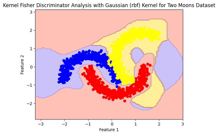
X, y = generate_three_moons()
linear#
model= Kfda(kernel='linear', n_components = 1)
model.fit(X,y)
Kfda(n_components=1)In a Jupyter environment, please rerun this cell to show the HTML representation or trust the notebook.
On GitHub, the HTML representation is unable to render, please try loading this page with nbviewer.org.
Kfda(n_components=1)
accuracy(model, X, y)
Accuracy: 0.68
plot_boundry_decision(model, X, y)
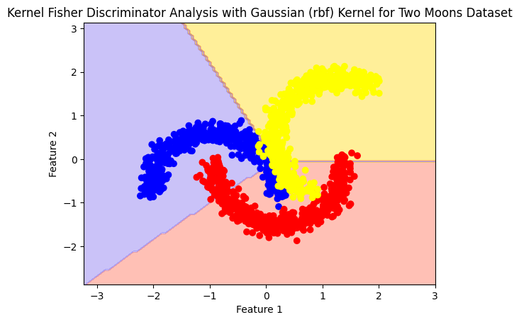
model= Kfda(kernel='linear', n_components = 2)
model.fit(X,y)
Kfda()In a Jupyter environment, please rerun this cell to show the HTML representation or trust the notebook.
On GitHub, the HTML representation is unable to render, please try loading this page with nbviewer.org.
Kfda()
from sklearn.metrics import accuracy_score
# Assuming you have already fit the model as follows:
# model = Kfda(kernel='linear', n_components=1)
# model.fit(X, y)

# Predict the labels on the same dataset
y_pred = model.predict(X)

# Calculate and print accuracy
acc = accuracy_score(y, y_pred)
print(f"Accuracy: {acc}")
Accuracy: 0.7946666666666666
plot_boundry_decision(model, X, y)
model= Kfda(kernel='linear', n_components = 3)
model.fit(X,y)
C:\Users\Hadi\AppData\Local\Temp\ipykernel_4304\3548760067.py:29: UserWarning: n_components > classes_.size - 1.Only the first classes_.size - 1 components will be valid.
  warnings.warn(
Kfda(n_components=3)In a Jupyter environment, please rerun this cell to show the HTML representation or trust the notebook.
On GitHub, the HTML representation is unable to render, please try loading this page with nbviewer.org.
Kfda(n_components=3)
from sklearn.metrics import accuracy_score
# Assuming you have already fit the model as follows:
# model = Kfda(kernel='linear', n_components=1)
# model.fit(X, y)

# Predict the labels on the same dataset
y_pred = model.predict(X)

# Calculate and print accuracy
acc = accuracy_score(y, y_pred)
print(f"Accuracy: {acc}")
Accuracy: 0.7946666666666666
plot_boundry_decision(model, X, y)
C:\Users\Hadi\AppData\Local\Temp\ipykernel_4304\3548760067.py:29: UserWarning: n_components > classes_.size - 1.Only the first classes_.size - 1 components will be valid.
  warnings.warn(

Polynomial#
polynomial_model= Kfda(kernel='polynomial')
polynomial_model.fit(X,y)
Kfda(kernel='polynomial')In a Jupyter environment, please rerun this cell to show the HTML representation or trust the notebook.
On GitHub, the HTML representation is unable to render, please try loading this page with nbviewer.org.
Kfda(kernel='polynomial')
from sklearn.metrics import accuracy_score
# Assuming you have already fit the model as follows:
# model = Kfda(kernel='linear', n_components=1)
# model.fit(X, y)

# Predict the labels on the same dataset
y_pred = model.predict(X)

# Calculate and print accuracy
acc = accuracy_score(y, y_pred)
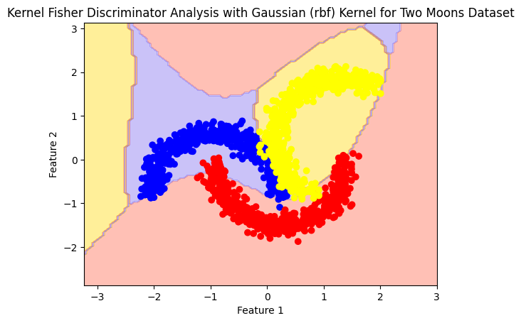
print(f"Accuracy: {acc}")
Accuracy: 0.666
plot_boundry_decision(polynomial_model, X, y)
RBF#
rbf_model= Kfda(kernel='rbf')
rbf_model.fit(X,y)
Kfda(kernel='rbf')In a Jupyter environment, please rerun this cell to show the HTML representation or trust the notebook.
On GitHub, the HTML representation is unable to render, please try loading this page with nbviewer.org.
Kfda(kernel='rbf')
from sklearn.metrics import accuracy_score
# Assuming you have already fit the model as follows:
# model = Kfda(kernel='linear', n_components=1)
# model.fit(X, y)

# Predict the labels on the same dataset
y_pred = model.predict(X)

# Calculate and print accuracy
acc = accuracy_score(y, y_pred)
print(f"Accuracy: {acc}")
Accuracy: 0.666
plot_boundry_decision(rbf_model, X, y)
