
Gaussian Process#
We examine the Gaussian process from both the weight-space and function-space perspectives.
Weight-space View#
Linear Model:#
\( x \) is the input vector.
\( w \) is the vector of weights (parameters) of the linear model.
\( f(x) \) is the function value.
\( y \) is the observed target value.
\( \epsilon \sim \mathcal{N}(0, \sigma^2_n) \) is the additive noise.
Likelihood:
\( y \) is the vector of observed target values.
\( X \) is the matrix of input vectors.
\( \sigma^2_n \) is the variance of the noise.
The likelihood \( p(y|X,w) \) represents the probability of observing \( y \) given \( X \) and \( w \).
Prior: $\( w \sim \mathcal{N}(0, \Sigma_p) \)$
A zero-mean Gaussian prior with covariance matrix \( \Sigma_p \) is placed on the weights \( w \).
Posterior:
The posterior distribution \( p(w|X,y) \) is Gaussian with mean \( \bar{w} \) and covariance matrix \( A^{-1} \).
\( \bar{w} = \left( \sigma^{-2}_n (XX^\top) + \Sigma_p^{-1} \right)^{-1} Xy \)
\( A = \sigma^{-2}_n XX^\top + \Sigma_p^{-1} \)
Predictive Distribution: $\( p(f_*|x_*,X,y) = \int p(f_*|x_*,w) p(w|X,y) \, dw \)\( \)\( = \mathcal{N}\left( \frac{1}{\sigma^2_n} x_*^\top A^{-1} Xy, x_*^\top A^{-1} x_* \right) \)$
The predictive distribution for \( f_* = f(x_*) \) at a new input \( x_* \) is obtained by averaging over all possible parameter values, weighted by their posterior probability.
import numpy as np
import matplotlib.pyplot as plt
# Generate synthetic data
np.random.seed(0)
x = np.linspace(-3, 3, 100)
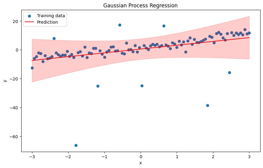
y = 2 + 3 * x + 0 * x**2 + np.random.normal(0, 2, x.shape)
# Introduce outliers
y[::10] += 120 * (np.random.rand(10) - 0.5)
# Linear model
def linear_model(X, w):
return X @ w
# Likelihood (not directly used in the code but provided for completeness)
def likelihood(y, X, w, sigma_n):
n = len(y)
pred = linear_model(X, w)
return (1 / (np.sqrt(2 * np.pi) * sigma_n)) ** n * np.exp(-np.sum((y - pred) ** 2) / (2 * sigma_n ** 2))
# Prior (not directly used in the code but provided for completeness)
def prior(w, Sigma_p):
d = len(w)
return (1 / np.sqrt((2 * np.pi) ** d * np.linalg.det(Sigma_p))) * np.exp(-0.5 * w.T @ np.linalg.inv(Sigma_p) @ w)
# Posterior
def posterior(X, y, sigma_n, Sigma_p):
y = y.reshape(-1, 1) # Ensure y is a column vector
A = (1 / sigma_n ** 2) * X.T @ X + np.linalg.inv(Sigma_p)
w_bar = np.linalg.inv(A) @ (X.T @ y) * (1 / sigma_n ** 2)
return w_bar, A
# Predictive distribution
def predict(X_train, y_train, X_test, sigma_n, Sigma_p):
w_bar, A = posterior(X_train, y_train, sigma_n, Sigma_p)
y_pred = X_test @ w_bar
pred_var = np.diag(X_test @ np.linalg.inv(A) @ X_test.T)
return y_pred.flatten(), pred_var
# Add bias term to the input
X_train = np.vstack([np.ones(x.shape), x]).T
y_train = y
# Define test points
x_test = np.linspace(-3, 3, 100)
X_test = np.vstack([np.ones(x_test.shape), x_test]).T
# Hyperparameters
sigma_n = 40
Sigma_p = 80*np.eye(X_train.shape[1])
# Fit and predict using Gaussian Process Regression
y_pred, pred_var = predict(X_train, y_train, X_test, sigma_n, Sigma_p)
# Plot the results
plt.figure(figsize=(10, 6))
plt.scatter(x, y, label='Training data')
plt.plot(x_test, y_pred, label='Prediction', color='red')
plt.fill_between(x_test, y_pred - 1.96 * np.sqrt(pred_var), y_pred + 1.96 * np.sqrt(pred_var), alpha=0.2, color='red')
plt.title('Gaussian Process Regression')
plt.xlabel('x')
plt.ylabel('y')
plt.legend()
plt.show()
Step-by-Step Implementation of GP#
Step 1: Generating Synthetic Data#
import numpy as np
import matplotlib.pyplot as plt

# Generate synthetic data
np.random.seed(0)
x = np.linspace(-3, 3, 100)
y = 2 + 3 * x + 0 * x**2 + np.random.normal(0, 2, x.shape)
Step 2: Define the Linear Model#
# Linear model
def linear_model(X, w):
    return X @ w
Step 3: Define the Likelihood#
def likelihood(y, X, w, sigma_n):
    n = len(y)
    pred = linear_model(X, w)
    return (1 / (np.sqrt(2 * np.pi) * sigma_n)) ** n * np.exp(-np.sum((y - pred) ** 2) / (2 * sigma_n ** 2))
Step 4: Define the Prior#
def prior(w, Sigma_p):
    d = len(w)
    return (1 / np.sqrt((2 * np.pi) ** d * np.linalg.det(Sigma_p))) * np.exp(-0.5 * w.T @ np.linalg.inv(Sigma_p) @ w)
Step 5: Compute the Posterior#
def posterior(X, y, sigma_n, Sigma_p):
    A = (1 / sigma_n ** 2) * X.T @ X + np.linalg.inv(Sigma_p)
    w_bar = np.linalg.inv(A) @ (1 / sigma_n ** 2) * X.T @ y
    return w_bar, A
Step 6: Define the Predictive Distribution#
def predict(X_train, y_train, X_test, sigma_n, Sigma_p):
    w_bar, A = posterior(X_train, y_train, sigma_n, Sigma_p)
    y_pred = X_test @ w_bar
    pred_var = np.diag(X_test @ np.linalg.inv(A) @ X_test.T)
    return y_pred, pred_var
Weight-space View : Nonlinear model#
As discussed in the Linearization section of the Pattern Recognition course under Regression (Linearization), we use the feature space \(\phi\) defined as the Transformed Feature Space: \(\phi(x) = [1, x, x^2, \ldots, x^k]\). This technique linearizes the problem, allowing us to continue using a linear model as explained in the above section.
Remember: Polynomial Linearization: Understanding and Application
Polynomial regression is a form of linear regression where the relationship between the independent variable \( x \) and the dependent variable \( y \) is modeled as an \( n \)-degree polynomial. Despite its non-linear appearance, polynomial regression is treated as a linear regression problem by transforming the feature space.
Key Concepts#
Polynomial Features:
Polynomial regression extends linear regression by including polynomial terms of the features.
For example, in a quadratic polynomial regression, the model can be expressed as:
\[ y = \beta_0 + \beta_1 x + \beta_2 x^2 + \epsilon \]For a cubic polynomial regression, it becomes:
\[ y = \beta_0 + \beta_1 x + \beta_2 x^2 + \beta_3 x^3 + \epsilon \]By creating polynomial features, the regression model learns more complex relationships.
Linearization:
Polynomial regression is a linear model in terms of the coefficients \(\beta\).
Although the features themselves are non-linear (e.g., \(x^2\) or \(x^3\)), the relationship between the transformed features and the target variable \(y\) remains linear.
Feature Transformation:
To handle polynomial regression, we transform the original feature vector \( x \) into a higher-dimensional feature space.
For a cubic polynomial, the feature vector \( x \) is transformed as follows:
\[\begin{split} \phi(x) = \begin{bmatrix} x^3 \\ x^2 \\ x \\ 1 \end{bmatrix} \end{split}\]This transformation allows us to apply linear regression methods to the polynomial feature space.
Practical Application#
Data Preparation:
Convert the original feature vector \( x \) into the polynomial feature space.
For example, for a cubic polynomial, use the transformation:
def polynomial_features(x):
    return np.hstack([x**3, x**2, x, np.ones_like(x)])
Regression Model:
The regression model can be applied to these polynomial features just like linear regression.
The regression coefficients are estimated based on these transformed features, and predictions are made in the same feature space.
Example Code:
Here’s how you can apply polynomial features and perform linear regression:
import numpy as np
import matplotlib.pyplot as plt
# Generate synthetic data
np.random.seed(0)
x = np.linspace(-3, 3, 100).reshape(-1, 1) # Ensure x is a column vector
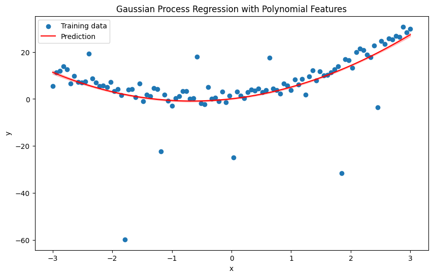
y = 2 + 3 * x + 2 * x**2 + np.random.normal(0, 2, (x.shape[0],1)) # y as a 1D array
#2 * x**2 - 3 * x + 5
# Introduce outliers
n_outliers = 10
outlier_indices = np.arange(0, len(x), len(x) // n_outliers)
y = y.flatten() # Convert y to 1D
y[outlier_indices] += 120 * (np.random.rand(len(outlier_indices)) - 0.5)
# Polynomial features transformation
def polynomial_features(x):
return np.hstack([x*x*x, x**2, x, np.ones_like(x)])
# Linear model
def linear_model(X, w):
return X @ w
# Posterior
def posterior(X, y, sigma_n, Sigma_p):
y = y.reshape(-1, 1) # Ensure y is a column vector
A = (1 / sigma_n ** 2) * (X.T @ X) + np.linalg.inv(Sigma_p)
w_bar = np.linalg.inv(A) @ (X.T @ y) # No need to multiply by (1 / sigma_n ** 2) here
return w_bar, A
# Predictive distribution
def predict(X_train, y_train, X_test, sigma_n, Sigma_p):
w_bar, A = posterior(X_train, y_train, sigma_n, Sigma_p)
y_pred = X_test @ w_bar
# Calculate predictive variance for each test point
pred_var = np.array([X_test[i, :] @ np.linalg.inv(A) @ X_test[i, :].T for i in range(X_test.shape[0])])
return y_pred.flatten(), pred_var.flatten()
# Prepare training and test data
X_train = polynomial_features(x) # Polynomial features for training
X_test = polynomial_features(np.linspace(-3, 3, 100).reshape(-1, 1)) # Same features for test
# Training data
y_train = y
# Hyperparameters
sigma_n = 0.99
Sigma_p = 1*np.eye(X_train.shape[1])
# Fit and predict using Gaussian Process Regression
y_pred, pred_var = predict(X_train, y_train, X_test, sigma_n, Sigma_p)
# Plot the results
plt.figure(figsize=(10, 6))
plt.scatter(x, y, label='Training data')
plt.plot(np.linspace(-3, 3, 100), y_pred, label='Prediction', color='red')
plt.fill_between(np.linspace(-3, 3, 100), y_pred - 1.96 * np.sqrt(pred_var), y_pred + 1.96 * np.sqrt(pred_var), alpha=0.2, color='red')
plt.title('Gaussian Process Regression with Polynomial Features')
plt.xlabel('x')
plt.ylabel('y')
plt.legend()
plt.show()
Homework 1#
Explore the multivariate weight-space view for both linear and nonlinear models. Write the necessary mathematical formulations and apply them using appropriate code on suitable data.
Function-Space View with Gaussian Processes#
In the function-space view, we use a Gaussian Process (GP) to describe a distribution over functions.
From \(\phi \) space (Feature space) to kernel-based covariance#
Projections of Inputs into Feature Space#
Feature Mapping:
The input vector \( x \) is projected into a feature space using a mapping \( \phi(x) \).
For example, a scalar input \( x \) can be mapped into the space of its powers: \(\phi(x) = (1, x, x^2, x^3, \ldots)^\top\).
Predictive Distribution in Feature Space:
The predictive distribution becomes: $\( f_* | x_*, X, y \sim \mathcal{N}\left( \frac{1}{\sigma^2_n} \phi(x_*)^\top A^{-1} \Phi y, \phi(x_*)^\top A^{-1} \phi(x_*) \right) \)$
Here, \(\Phi = \Phi(X)\) is the matrix of feature vectors of the training data.
\(A = \sigma^{-2}_n \Phi \Phi^\top + \Sigma_p^{-1}\).
Kernel Trick#
To address the computational challenge, we use the kernel trick:
Rewriting the Predictive Distribution:
The predictive distribution can be rewritten using the kernel trick: $\( f_* | x_*, X, y \sim \mathcal{N}\left( \phi_*^\top \Sigma_p \Phi (K + \sigma^2_n I)^{-1} y, \phi_*^\top \Sigma_p \phi_* - \phi_*^\top \Sigma_p \Phi (K + \sigma^2_n I)^{-1} \Phi^\top \Sigma_p \phi_* \right) \)$
Here, \(\phi_* = \phi(x_*)\) and \(K = \Phi^\top \Sigma_p \Phi\).
Covariance Function (Kernel)#
Inner Products in Feature Space:
The feature space enters the equations in the form of \(\Phi^\top \Sigma_p \Phi\), \(\phi_*^\top \Sigma_p \Phi\), or \(\phi_*^\top \Sigma_p \phi_*\).
These entries are inner products \(\phi(x)^\top \Sigma_p \phi(x')\) where \(x\) and \(x'\) are in the training or test sets.
Kernel Definition:
Define the kernel function \(k(x, x') = \phi(x)^\top \Sigma_p \phi(x')\).
This kernel function is also known as a covariance function.
Function-Space View with Gaussian Processes#
In the function-space view, we use a Gaussian Process (GP) to describe a distribution over functions. Mean and Covariance Functions:
The mean function \(m(x)\) and the covariance function \(k(x,x')\) of a real process \(f(x)\) are defined as:
\[ m(x) = \mathbb{E}[f(x)] \]\[ k(x, x') = \mathbb{E}[(f(x) - m(x))(f(x') - m(x'))] \]A Gaussian process can be written as:
\[ f(x) \sim \mathcal{GP}(m(x), k(x, x')) \]
Zero Mean Function:
For simplicity, the mean function is often taken to be zero:
\[ m(x) = 0 \]
Random Variables in GPs:
In this context, the random variables represent the value of the function \(f(x)\) at location \(x\). The index set \(X\) is the set of possible inputs.
Example: Bayesian Linear Regression:
Consider a Bayesian linear regression model \(f(x) = \phi(x)^\top w\) with prior \(w \sim \mathcal{N}(0, \Sigma_p)\). For this model:
\[ \mathbb{E}[f(x)] = \phi(x)^\top \mathbb{E}[w] = 0 \]\[ \mathbb{E}[f(x) f(x')] = \phi(x)^\top \mathbb{E}[w w^\top] \phi(x') = \phi(x)^\top \Sigma_p \phi(x') \]The covariance function specifies the covariance between pairs of random variables: $\( \text{cov}(f(x_p), f(x_q)) = k(x_p, x_q) = \exp\left( -\frac{1}{2} |x_p - x_q|^2 \right) \)$
Incorporate Observational Noise#
Assume we have noisy observations \( y_i = f(x_i) + \epsilon_i \) where \(\epsilon_i \sim \mathcal{N}(0, \sigma^2)\). The noise variance \(\sigma^2\) is added to the diagonal of the covariance matrix:
Joint Distribution of Training and Test Points
Consider a new test input \( x_* \). The joint distribution of the observed targets \(\mathbf{y}\) and the function value \( f_* = f(x_*) \) at \( x_* \) is:
where \(\mathbf{k}_* = [k(x_1, x_*), k(x_2, x_*), \ldots, k(x_N, x_*)]^T\) is the covariance vector between the training inputs and the test input.
Conditional Distribution for Predictions
Or
Prediction with Gaussian Processes#
The predictive distribution \( p(f_* | \mathbf{X}, \mathbf{y}, x_*) \) can be derived using the properties of multivariate Gaussian distributions. The conditional distribution of \( f_* \) given \(\mathbf{y}\) is:
where the mean and variance are given by:
Do works#
The six steps for Gaussian Process regression:
Define the Gaussian Process: \( f(x) \sim \mathcal{GP}(0, k(x, x')) \)
Specify the Kernel Function: Commonly used kernels include the RBF kernel.
Formulate the Joint Distribution: \(\mathbf{f} \sim \mathcal{N}(\mathbf{0}, \mathbf{K})\)
Incorporate Observational Noise: \(\mathbf{y} \sim \mathcal{N}(\mathbf{0}, \mathbf{K} + \sigma^2 \mathbf{I})\)
Joint Distribution of Training and Test Points: \(\begin{bmatrix} \mathbf{y} \\ f_* \end{bmatrix} \sim \mathcal{N} \left( \mathbf{0}, \begin{bmatrix} \mathbf{K} + \sigma^2 \mathbf{I} & \mathbf{k}_* \\ \mathbf{k}_*^T & k(x_*, x_*) \end{bmatrix} \right)\)
Conditional Distribution for Predictions:
Mean: \( \mu_* = \mathbf{k}_*^T (\mathbf{K} + \sigma^2 \mathbf{I})^{-1} \mathbf{y} \)
Variance: \( \sigma_*^2 = k(x_*, x_*) - \mathbf{k}_*^T (\mathbf{K} + \sigma^2 \mathbf{I})^{-1} \mathbf{k}_* \)
Function Space view of Gaussian Processes offer a flexible and powerful way and non-parametric method to model complex, non-linear relationships while providing probabilistic predictions with associated uncertainties.
Algorithm for GP-based Prediction#
Input: \(X\) (training inputs), \(y\) (training targets), \(k\) (covariance function), \(\sigma_n^2\) (noise level), \(x_*\) (test input)
Compute the Cholesky decomposition: \(L := \text{cholesky}(K + \sigma_n^2 I)\)
Solve for \(\alpha\): \(\alpha := L^\top \backslash (L \backslash y)\)
Compute the predictive mean: \(\bar{f}_* := k_*^\top \alpha\)
Compute the intermediate variable \(v\): \(v := L \backslash k_*\)
Compute the predictive variance: \(\text{Var}[f_*] := k(x_*, x_*) - v^\top v\)
Output: \(\bar{f}_*\) (mean), \(\text{Var}[f_*]\) (variance)
Calculating the Log Marginal Likelihood using \(\alpha\) and \(L\)#
The log marginal likelihood of the observed data \(y\) given the inputs \(X\) under the Gaussian process model is:
Homework 1#
What is the relationship between complexity and the term \( \sum_i \log L_{ii} \), and model fit and the term \( y^\top \alpha \)?” Also, change the points (in the following code) for training and testing, and adjust the parameters. Then, explain what occurs.
Implementation of GP prediction#
import numpy as np
import matplotlib.pyplot as plt
# Define the RBF kernel
def rbf_kernel(X1, X2, length_scale=1.0):
sqdist = np.sum(X1**2, 1).reshape(-1, 1) + np.sum(X2**2, 1) - 2 * np.dot(X1, X2.T)
return np.exp(-0.5 / length_scale**2 * sqdist)
# Training data (inputs and outputs)
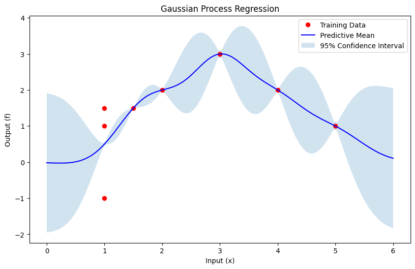
X_train = np.array([[1], [2], [3], [4], [5], [1.0],[1.5], [1]])
y_train = np.array([1, 2, 3, 2, 1, 1.5, 1.5, -1])
# Test data (inputs)
X_test = np.linspace(0, 6, 100).reshape(-1, 1)
length_scale=0.5
# Compute the covariance matrices
K = rbf_kernel(X_train, X_train, length_scale)
K_s = rbf_kernel(X_train, X_test, length_scale)
K_ss = rbf_kernel(X_test, X_test, length_scale)
sigma_n = 0.01 # Noise level
# Compute the Cholesky decomposition
L = np.linalg.cholesky(K + sigma_n**2 * np.eye(len(X_train)))
# Solve for alpha
alpha = np.linalg.solve(L.T, np.linalg.solve(L, y_train))
# Predictive mean
mean_s = np.dot(K_s.T, alpha)
# Solve for v
v = np.linalg.solve(L, K_s)
# Predictive variance
var_s = np.diag(K_ss) - np.sum(v**2, axis=0)
std_s = np.sqrt(var_s)
# Plotting
plt.figure(figsize=(10, 6))
plt.plot(X_train, y_train, 'ro', label='Training Data')
plt.plot(X_test, mean_s, 'b-', label='Predictive Mean')
plt.fill_between(X_test.ravel(), mean_s - 1.96 * std_s, mean_s + 1.96 * std_s, alpha=0.2, label='95% Confidence Interval')
plt.xlabel('Input (x)')
plt.ylabel('Output (f)')
plt.title('Gaussian Process Regression')
plt.legend()
plt.show()
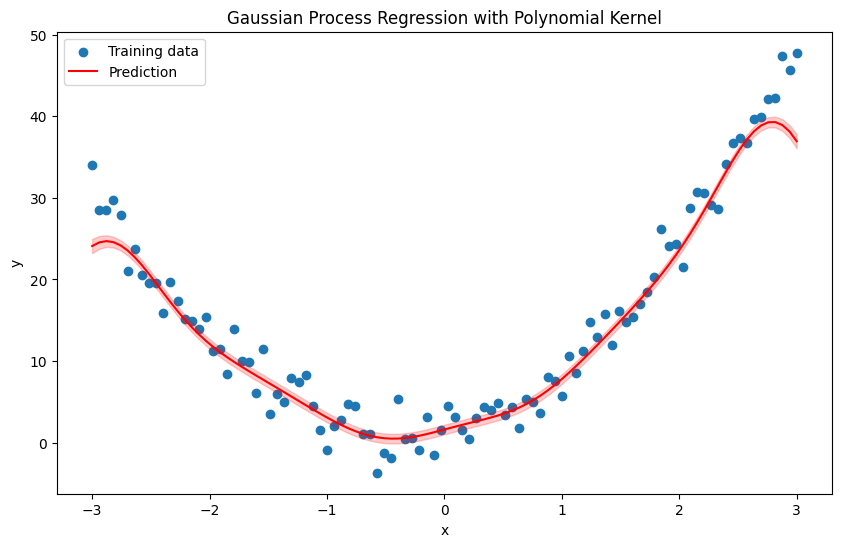
Polynomial Kernel Function#
where:
\(x_i\) and \(x_j\) are input vectors.
\(c\) is a constant.
\(d\) is the degree of the polynomial.
import numpy as np
import matplotlib.pyplot as plt
# Generate synthetic data
np.random.seed(0)
x = np.linspace(-3, 3, 100)
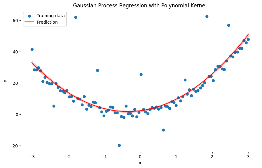
y = 2 + 3 * x + 4 * x**2 + np.random.normal(0, 2, x.shape)
# Remove outliers for simplicity
y[::10] -= 120 * (np.random.rand(10) - 0.5)
# Add bias term to the input
X_train = x.reshape(-1, 1) # Train input matrix
y_train = y
# Polynomial kernel function
def polynomial_kernel(X1, X2, c=1.0, d=2):
return (X1 @ X2.T + c) ** d
# Compute the covariance matrices
def compute_covariances(X_train, X_test, sigma_n):
K_train_train = polynomial_kernel(X_train, X_train)
K_test_train = polynomial_kernel(X_test, X_train)
K_test_test = polynomial_kernel(X_test, X_test)
K_train_train += sigma_n ** 2 * np.eye(X_train.shape[0]) # Add noise variance to the training covariance matrix
return K_train_train, K_test_train, K_test_test
# Predictive distribution
def predict(X_train, y_train, X_test, sigma_n):
K_train_train, K_test_train, K_test_test = compute_covariances(X_train, X_test, sigma_n)
# Compute the mean of the predictive distribution
K_train_train_inv = np.linalg.inv(K_train_train)
mean = K_test_train @ K_train_train_inv @ y_train
# Compute the covariance of the predictive distribution
covariance = K_test_test - K_test_train @ K_train_train_inv @ K_test_train.T
return mean.flatten(), np.diag(covariance)
# Define test points
x_test = np.linspace(-3, 3, 100).reshape(-1, 1)
X_test = x_test
# Hyperparameters
sigma_n = 2.0 # Noise variance
# Fit and predict using Gaussian Process Regression
y_pred, pred_var = predict(X_train, y_train, X_test, sigma_n)
# Plot the results
plt.figure(figsize=(10, 6))
plt.scatter(x, y, label='Training data')
plt.plot(x_test, y_pred, label='Prediction', color='red')
plt.fill_between(x_test.flatten(), y_pred - 1.96 * np.sqrt(pred_var), y_pred + 1.96 * np.sqrt(pred_var), alpha=0.2, color='red')
plt.title('Gaussian Process Regression with Polynomial Kernel')
plt.xlabel('x')
plt.ylabel('y')
plt.legend()
plt.show()
Again above example with RBF kernel#
import numpy as np
import matplotlib.pyplot as plt

# Generate synthetic data
np.random.seed(0)
x = np.linspace(-3, 3, 100)
y = 2 + 3 * x + 4 * x**2 + np.random.normal(0, 2, x.shape)

# Remove outliers for simplicity
y[::10] -= 20 * (np.random.rand(10) - 0.5)

# Add bias term to the input
X_train = x.reshape(-1, 1)  # Train input matrix
y_train = y

# Define the RBF kernel
def rbf_kernel(X1, X2, length_scale=1.0):
    sqdist = np.sum(X1**2, 1).reshape(-1, 1) + np.sum(X2**2, 1) - 2 * np.dot(X1, X2.T)
    return np.exp(-0.5 / length_scale**2 * sqdist)

# Compute the covariance matrices
def compute_covariances(X_train, X_test, sigma_n, length_scale):
    K_train_train = rbf_kernel(X_train, X_train, length_scale)
    K_test_train = rbf_kernel(X_test, X_train, length_scale)
    K_test_test = rbf_kernel(X_test, X_test, length_scale)
    K_train_train += sigma_n ** 2 * np.eye(X_train.shape[0])  # Add noise variance to the training covariance matrix
    return K_train_train, K_test_train, K_test_test

# Predictive distribution
def predict(X_train, y_train, X_test, sigma_n, length_scale):
    K_train_train, K_test_train, K_test_test = compute_covariances(X_train, X_test, sigma_n, length_scale)

    # Compute the mean of the predictive distribution
    K_train_train_inv = np.linalg.inv(K_train_train)
    mean = K_test_train @ K_train_train_inv @ y_train

    # Compute the covariance of the predictive distribution
    covariance = K_test_test - K_test_train @ K_train_train_inv @ K_test_train.T

    return mean.flatten(), np.diag(covariance)


# Define test points
x_test = np.linspace(-3, 3, 100).reshape(-1, 1)
X_test = x_test

# Hyperparameters
sigma_n = 1.0  # Noise variance
length_scale=0.5

# Fit and predict using Gaussian Process Regression
y_pred, pred_var = predict(X_train, y_train, X_test, sigma_n, length_scale)

# Plot the results
plt.figure(figsize=(10, 6))
plt.scatter(x, y, label='Training data')
plt.plot(x_test, y_pred, label='Prediction', color='red')
plt.fill_between(x_test.flatten(), y_pred - 1.96 * np.sqrt(pred_var), y_pred + 1.96 * np.sqrt(pred_var), alpha=0.2, color='red')
plt.title('Gaussian Process Regression with Polynomial Kernel')
plt.xlabel('x')
plt.ylabel('y')
plt.legend()
plt.show()
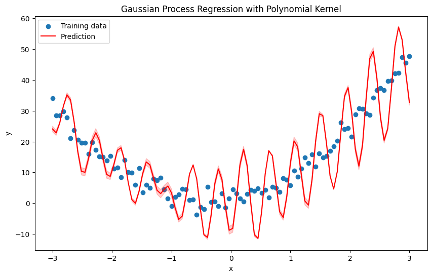
RBF with \(\epsilon \) Insensitive Loss#
import numpy as np
import matplotlib.pyplot as plt

def epsilon_loss(preds, target, epsilon=0.1):
    n1 = len(preds)
    n2 = len(target)
    K = np.zeros((n1, n2))

    for i in range(n1):
        for j in range(n2):
            errors = np.abs(target[i] - preds[j])
            loss = np.maximum(0, errors - epsilon)
            K[i, j] = 4 * loss**2
    return K

def rbf_kernel(x1, x2, length_scale=1.0, sigma_f=1.0, epsilon=0.1):
    sqdist = epsilon_loss(x1, x2, epsilon)
    return sigma_f**2 * np.exp(-0.5 / length_scale**2 * sqdist)


# # Define the RBF kernel
# def rbf_kernel(X1, X2, length_scale=1.0):
#     sqdist = np.sum(X1**2, 1).reshape(-1, 1) + np.sum(X2**2, 1) - 2 * np.dot(X1, X2.T)
#     return np.exp(-0.5 / length_scale**2 * sqdist)

# Compute the covariance matrices
def compute_covariances(X_train, X_test, sigma_n, length_scale, epsilon):
    K_train_train = rbf_kernel(X_train, X_train, length_scale, epsilon)
    K_test_train = rbf_kernel(X_test, X_train, length_scale, epsilon)
    K_test_test = rbf_kernel(X_test, X_test, length_scale, epsilon)
    K_train_train += sigma_n ** 2 * np.eye(X_train.shape[0])  # Add noise variance to the training covariance matrix
    return K_train_train, K_test_train, K_test_test

# Predictive distribution
def predict(X_train, y_train, X_test, sigma_n, length_scale, epsilon):
    K_train_train, K_test_train, K_test_test = compute_covariances(X_train, X_test, sigma_n, length_scale, epsilon)

    # Compute the mean of the predictive distribution
    K_train_train_inv = np.linalg.inv(K_train_train)
    mean = K_test_train @ K_train_train_inv @ y_train

    # Compute the covariance of the predictive distribution
    covariance = K_test_test - K_test_train @ K_train_train_inv @ K_test_train.T

    return mean.flatten(), np.diag(covariance)


# Generate synthetic data
np.random.seed(0)
x = np.linspace(-3, 3, 100)
y = 2 + 3 * x + 4 * x**2 + np.random.normal(0, 2, x.shape)

# Remove outliers for simplicity
y[::10] -= 20 * (np.random.rand(10) - 0.5)

# Add bias term to the input
X_train = x.reshape(-1, 1)  # Train input matrix
y_train = y

# Define test points
x_test = np.linspace(-3, 3, 100).reshape(-1, 1)
X_test = x_test

# Hyperparameters
sigma_n = 1.0  # Noise variance
length_scale=0.5
epsilon= 2
# Fit and predict using Gaussian Process Regression
y_pred, pred_var = predict(X_train, y_train, X_test, sigma_n, length_scale, epsilon)

# Plot the results
plt.figure(figsize=(10, 6))
plt.scatter(x, y, label='Training data')
plt.plot(x_test, y_pred, label='Prediction', color='red')
plt.fill_between(x_test.flatten(), y_pred - 1.96 * np.sqrt(pred_var), y_pred + 1.96 * np.sqrt(pred_var), alpha=0.2, color='red')
plt.title('Gaussian Process Regression with Polynomial Kernel')
plt.xlabel('x')
plt.ylabel('y')
plt.legend()
plt.show()
C:\Users\Hadi\AppData\Local\Temp\ipykernel_3688\3957923635.py:13: DeprecationWarning: Conversion of an array with ndim > 0 to a scalar is deprecated, and will error in future. Ensure you extract a single element from your array before performing this operation. (Deprecated NumPy 1.25.)
  K[i, j] = 4 * loss**2
C:\Users\Hadi\AppData\Local\Temp\ipykernel_3688\3957923635.py:76: RuntimeWarning: invalid value encountered in sqrt
  plt.fill_between(x_test.flatten(), y_pred - 1.96 * np.sqrt(pred_var), y_pred + 1.96 * np.sqrt(pred_var), alpha=0.2, color='red')
Homework 2#
Preface
Discussion on RBF Kernel with \(\epsilon\)-Insensitive Loss
In Homework 2, we examined the Radial Basis Function (RBF) kernel and its integration with the \(\epsilon\)-Insensitive Loss function. This analysis provides insight into how different components of a machine learning model interact, specifically in the context of Gaussian Processes (GPs) and Support Vector Regression.
Radial Basis Function (RBF) Kernel:
The RBF kernel, also known as the Gaussian kernel, is defined as:
\[ k(x_i, x_j) = \sigma_f^2 \exp\left(-\frac{\|x_i - x_j\|^2}{2 \ell^2}\right) \]where \( \sigma_f^2 \) is the signal variance, and \( \ell \) is the length scale parameter.
Properties:
Locality: The RBF kernel measures similarity based on the distance between points, with closer points being more similar.
Smoothness: Functions modeled with the RBF kernel are smooth and infinitely differentiable.
Application in GPs:
In Gaussian Processes, the RBF kernel is used to define the covariance function between pairs of data points. It determines how the model smooths and interpolates data.
\(\epsilon\)-Insensitive Loss:
This loss function is commonly used in Support Vector Regression (SVR) and is defined as:
\[\begin{split} L_\epsilon(y, f(x)) = \begin{cases} 0 & \text{if } |y - f(x)| \leq \epsilon \\ |y - f(x)| - \epsilon & \text{otherwise} \end{cases} \end{split}\]where \( \epsilon \) is a parameter that specifies a tolerance zone around the prediction \( f(x) \).
Application in SVR:
Fit Term: The \(\epsilon\)-Insensitive Loss function ensures that predictions within an \(\epsilon\) margin around the observed data \( y \) incur no loss. This helps in focusing the learning on the points where the prediction deviates significantly from the true value.
Robustness: By ignoring errors within the \(\epsilon\) margin, the model becomes less sensitive to outliers and noise in the data.
Now You Complete
Integration of RBF Kernel and \(\epsilon\)-Insensitive Loss
Multivariate form
Mathematical formulation & experiments
Mastery over the regulation of \(\epsilon\) in the synthetic example above
Applied to suitable applications that need the \(\epsilon\)-insensitive property