Locally Linear Embedding (LLE)#
Manifold learning
Preliminaries#
Neighborhoods#
Small group of houses in the immediate vicinity of one’s house or to a larger area with similar housing types and market values
For you in Iran, Mashhad
and you in London
Open Sets: Think of open sets as neighborhoods.
Topological Space from the Perspective of Neighborhoods#
In topology, we want to describe how points in a space are related to each other in terms of “closeness” or “nearness” without using distance. One powerful way to do this is through the concept of neighborhoods.
What is a Neighborhood?#
A neighborhood of a point \( p \) (think your house) in a topological space is a set that includes \( p \) and contains points (father house) that we consider “close” to \( p \). Importantly, a neighborhood isn’t defined by how far away these points are from \( p \) but rather by a more abstract sense of inclusion.
Open Neighborhood: An open neighborhood of a point \( p \) is simply a set that contains \( p \) and is part of the larger structure we call open sets. This open set is a way to group points that are near each other.
Neighborhoods Instead of Distance#
In standard geometry, we often say that two points are close because they have a small distance between them. In topology, instead of measuring distance, we say that two points are close if one point is within the neighborhood of the other.
No Distance, Just Inclusion: Rather than using a number to describe how close two points are, we use neighborhoods to capture the idea of closeness. If point \( p \) is in a neighborhood that includes point \( q \), we can think of \( p \) (your house) and \( q \) (house of your brother) as being close.
Example: Neighborhoods on the interval number#
Imagine the interval number:
In standard geometry, you could measure the distance between two points, like 2 and 3.
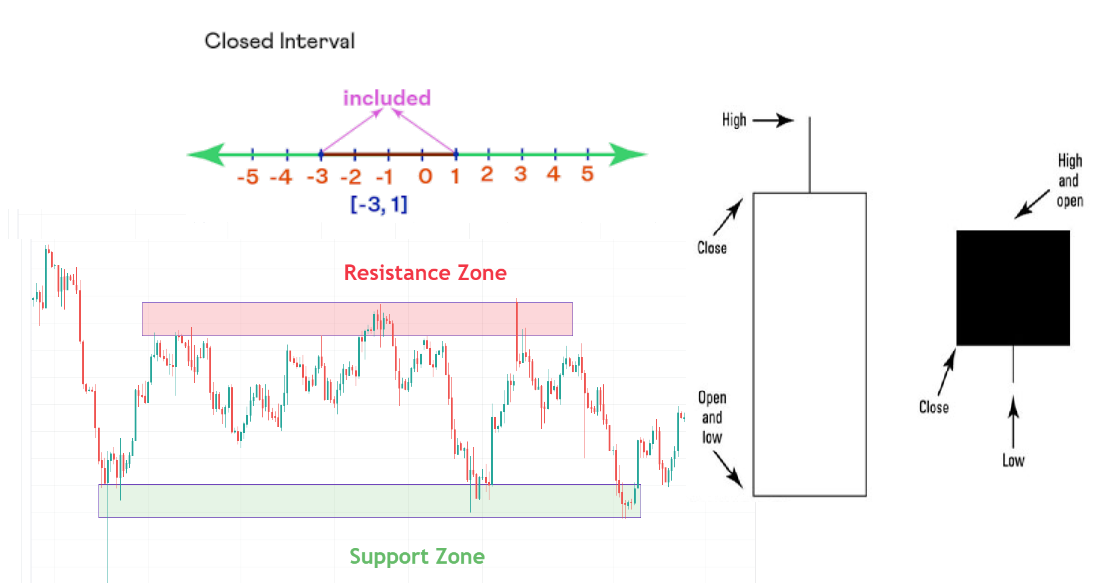
In topology, you could define a neighborhood around the point 2, like the interval \((1.5, 2.5)\). This interval is a neighborhood of 2 because it includes points that we consider near 2, but we never specify how near in terms of distance.
The point 3 could be in the neighborhood of another point, like \((2.5, 3.5)\), but 2 and 3 might not share the same neighborhood.
Why Use Neighborhoods?#
Flexibility: Neighborhoods allow us to describe how points are related without needing to define an exact distance. This is useful in spaces where distance doesn’t make sense or isn’t practical to use.
Generalization: Using neighborhoods, we can describe a wide range of spaces, including those that are more abstract or complex than our familiar Euclidean spaces.
Example in Practice: Sphere Surface#
Think about the surface of a sphere:
In topology, we might not talk about the distance between two points on the sphere. Instead, we discuss neighborhoods around a point, like small patches on the surface.
Two points are close if their neighborhoods overlap or are contained within a larger neighborhood.
Manifold from the Perspective of Neighborhoods#
A manifold is a special kind of topological space that, although it can have a complex, curved shape globally, looks like ordinary Euclidean space when you zoom in close enough. This means that for any point on a manifold, there exists a neighborhood around that point which resembles a familiar, flat Euclidean space.
What is a Manifold?#
A manifold is a topological space that satisfies the following properties:
Locally Euclidean: Every point on a manifold has a neighborhood that looks like a piece of \( \mathbb{R}^n \) (Euclidean space of dimension \( n \)). This means that even though the manifold might be curved or have a complicated global structure, small enough neighborhoods around any point look flat and simple, just like a small patch of the Earth’s surface appears flat even though the Earth is round.
Coordinate Systems (Charts): Each of these neighborhoods can be described using a local coordinate system, called a chart. These coordinates work just like the familiar \( x, y, z \) coordinates in Euclidean space, but only within the neighborhood.
Transition Maps: When you move from one neighborhood to another on the manifold, the coordinates might change. The rules for changing from one set of coordinates to another are called transition maps. These maps ensure that different coordinate systems fit together smoothly.
Extending the Neighborhood Concept#
In a topological space, neighborhoods help us understand how points relate to each other without using distance. In a manifold, neighborhoods do the same thing but with an extra twist: each neighborhood not only shows us “closeness” but also looks like part of a Euclidean space.
Local Flatness: Consider a point \( p \) on a manifold. The neighborhood around \( p \) is not just any abstract set; it looks and behaves like a small piece of flat Euclidean space. This means that, locally, the manifold “feels” flat, even if it might be curved when viewed as a whole.
Example: Sphere as a Manifold: Take the surface of a sphere. Globally, it’s curved, but if you zoom in on a small neighborhood around any point, that neighborhood looks flat, like a small piece of a plane. In this neighborhood, you can use coordinates like latitude and longitude to describe locations, similar to how you use \( x, y \) coordinates in a plane.
Why Manifolds Matter#
Some example:
Curved Surfaces: The surface of a sphere, the shape of a torus, or more complex surfaces can all be described as manifolds. Each of these surfaces, though curved globally, can be understood locally using flat, Euclidean neighborhoods.
Think of the Earth as a manifold:
Locally Flat: Any small neighborhood on the Earth’s surface, like a town or a city, looks flat. You can use a map with \( x, y \) coordinates to navigate, just as you would on a piece of paper. Each piece specified by latitude and longitude
Result: A manifold is a topological space that is locally Euclidean#
What is Manifold Learning?#
Manifold Hypothesis: This is the idea that real-world high-dimensional data often resides on a low-dimensional manifold. For example, images of faces might be described by hundreds of pixels (dimensions), but the variations in those images (like expressions or lighting) might only involve a few underlying factors, such as the position of the eyes, mouth, or the angle of the face. These underlying factors form a low-dimensional manifold within the high-dimensional pixel space.
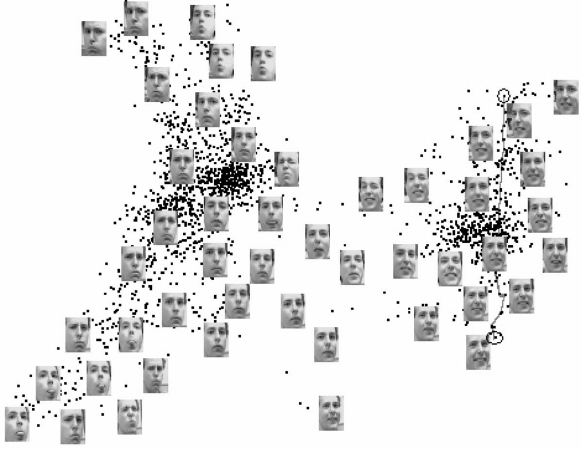
Interpretation of Points and Faces
Each Point Represents a Face: In this 2D visualization, each point corresponds to one face image from your dataset. The position of each point in the 2D space is determined by the similarities and differences in the facial features captured by the high-dimensional data. Faces that are similar in appearance (e.g., similar expressions, lighting conditions, or angles) tend to be mapped closer to each other in this 2D space.
Manifold (Clusters of Points): Points that are close together in this 2D space likely represent faces with similar characteristics. For example, a cluster of points might represent faces that all have a similar lighting condition or a similar expression like anger. This clustering happens because manifold learning preserves the local structure of the data, meaning that faces with similar high-dimensional features are kept close together in the lower-dimensional representation.
Manifolds of MNIST
Some of types of manifold learning methods#
Principal Component Analysis (PCA): Linear method for reducing dimensions by maximizing variance.
Multidimensional Scaling (MDS): Preserves pairwise distances when mapping to lower dimensions.
Isomap: Nonlinear method that preserves geodesic distances on the manifold.
Locally Linear Embedding (LLE): Captures local linear relationships between data points.
Laplacian Eigenmaps: Uses graph-based approach to preserve local neighborhood similarities.
t-Distributed Stochastic Neighbor Embedding (t-SNE): Visualizes data by preserving local similarities and revealing clusters.
Uniform Manifold Approximation and Projection (UMAP): Fast method that preserves both local and global structures in data.
Autoencoders: Neural networks that learn a low-dimensional representation through encoding and decoding.
We previously discussed PCA and autoencoders. Now, let’s introduce Locally Linear Embedding (LLE).
Locally Linear Embedding (LLE) Algorithm#
LLE is a nonlinear dimensionality reduction technique that aims to preserve local linear relationships within the data. It assumes that data points are samples from a smooth manifold, and the local patches around each point can be approximated linearly.
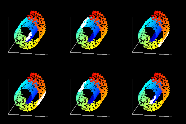
Nearest Neighbor Identification:
Goal: For each data point \( \mathbf{x}_i \), identify its \( k \) nearest neighbors using a distance metric (typically Euclidean).
Purpose: These neighbors define a local linear patch of the manifold around \( \mathbf{x}_i \).
Reconstruction Weights:
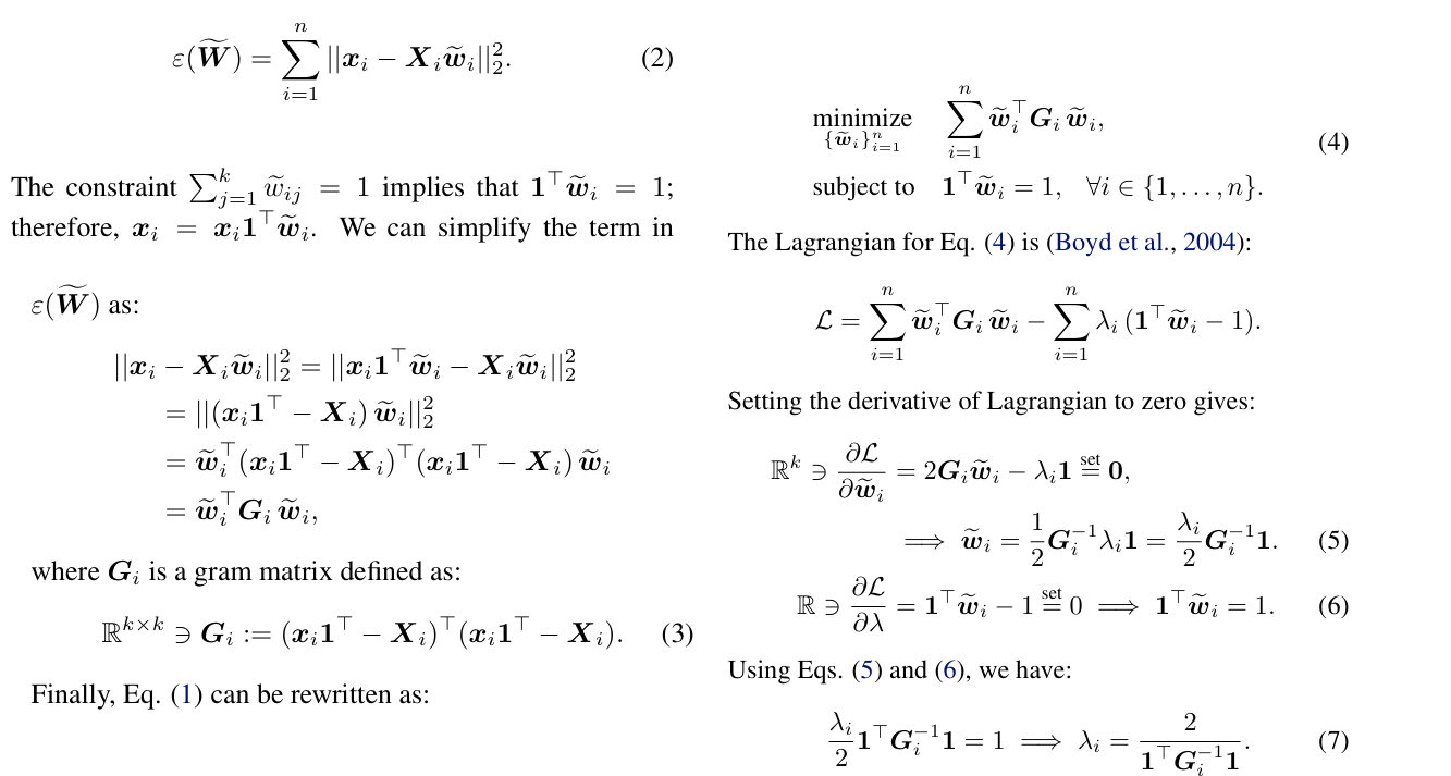
Objective: Find weights \( W_{ij} \) that best reconstruct each data point \( \mathbf{x}_i \) from its \( k \) neighbors \( \mathbf{x}_j \).
Cost Function: Minimize the reconstruction error:
where \( \mathcal{N}(i) \) is the set of \( k \) nearest neighbors of \( \mathbf{x}_i \), and \( W_{ij} \) are the reconstruction weights.
Constraints:
Reconstruction Constraint: Each data point is reconstructed from its neighbors.
Sum-to-One Constraint: Weights must sum to one:
Optimization: Solve the least-squares problem with these constraints to find the optimal weights \( W_{ij} \).
Embedding Cost Function#
After finding the optimal reconstruction weights \( W_{ij} \), the LLE algorithm maps the high-dimensional data into a lower-dimensional space while preserving local linear relationships. This step involves minimizing a cost function related to the reconstruction weights.
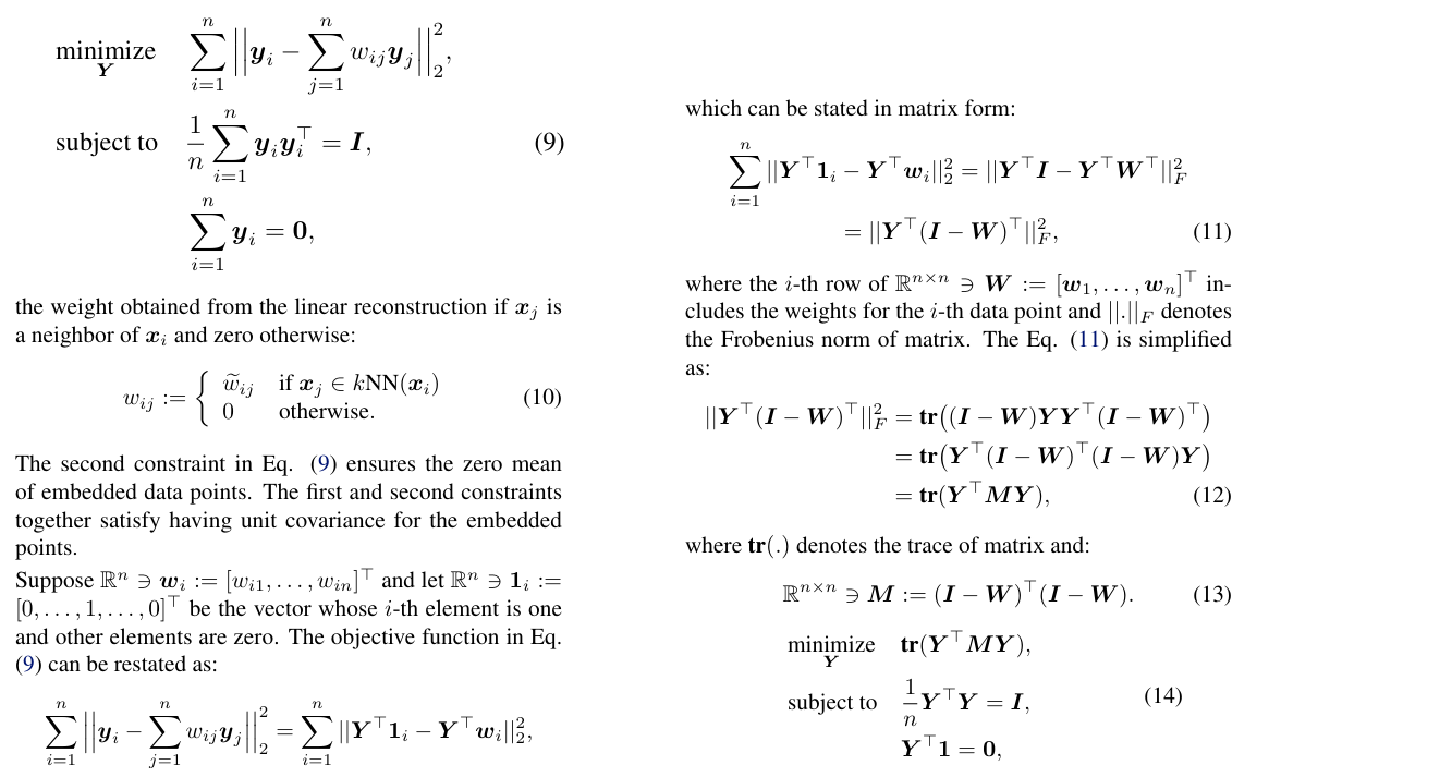
Reconstruction Weight Matrix: Given the weights \( W_{ij} \) from the high-dimensional space, you want to find low-dimensional coordinates \( \mathbf{y}_i \) that best preserve the local structure defined by these weights.
Cost Function: The embedding cost function is:
where:
\( \mathbf{y}_i \) is the low-dimensional representation of \( \mathbf{x}_i \).
\( W_{ij} \) are the weights computed in the previous step.
\( \mathcal{N}(i) \) is the set of \( k \) nearest neighbors of \( \mathbf{x}_i \) in the high-dimensional space.
Constraints: To ensure a meaningful embedding, the following constraints are applied:
Zero Mean Constraint: The coordinates \( \mathbf{y}_i \) should be centered:
This ensures that the embedding is centered around the origin.
Orthogonality Constraint: The coordinates should be orthogonal:
where \( \mathbf{Y} \) is the matrix of low-dimensional coordinates, and \( I \) is the identity matrix. This constraint ensures that the low-dimensional space is properly scaled and the dimensions are orthogonal.
Homework: Complete the details on the mathematics of Locally Linear Embedding (LLE).#
See Locally Linear Embedding and its Variants: Tutorial and Survey
More details#
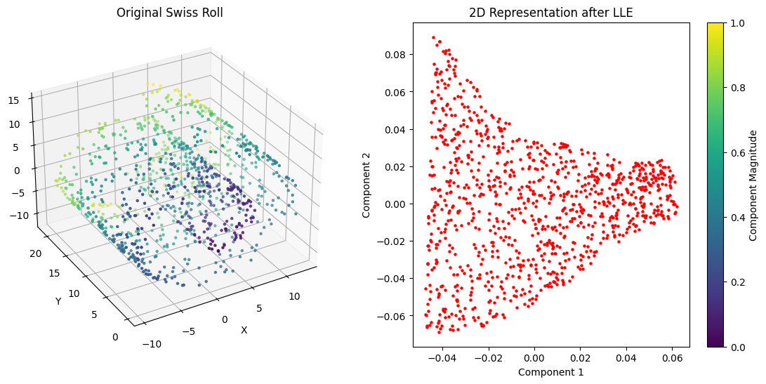
import numpy as np
import matplotlib.pyplot as plt
from mpl_toolkits.mplot3d import Axes3D
from sklearn.datasets import make_swiss_roll
from sklearn.manifold import LocallyLinearEmbedding

# Generate synthetic Swiss Roll data
X, _ = make_swiss_roll(n_samples=1000, noise=0.1, random_state=42)

# Apply LLE for dimensionality reduction
lle = LocallyLinearEmbedding(n_neighbors=10, n_components=2)
X_reduced = lle.fit_transform(X)

# Plot the original Swiss Roll as a surface
fig = plt.figure(figsize=(14, 6))

# 3D surface plot of the original Swiss Roll
ax1 = fig.add_subplot(121, projection='3d')
ax1.scatter(X[:, 0], X[:, 1], X[:, 2], c=np.sqrt(X[:, 0]**2 + X[:, 1]**2 + X[:, 2]**2), cmap='viridis', s=5)
ax1.set_title('Original Swiss Roll')
ax1.set_xlabel('X')
ax1.set_ylabel('Y')
ax1.set_zlabel('Z')
ax1.view_init(elev=30, azim=240)

# 2D plot of the reduced Swiss Roll
ax2 = fig.add_subplot(122)
sc = ax2.scatter(X_reduced[:, 0], X_reduced[:, 1], c='red', s=5)
ax2.set_title('2D Representation after LLE')
ax2.set_xlabel('Component 1')
ax2.set_ylabel('Component 2')

plt.colorbar(sc, ax=ax2, label='Component Magnitude')

plt.show()
