Signal Definition

Signal Definition#

A signal is a function of one or more variables that describes a phenomenon.

Continuous-time signal $x(t)$ or analog:
A continuous signal has continuous argument(s). For example, a signal with one argument $x(t)$:

\[ x(t) : \mathbb{R} \to \mathbb{R} \]

Or, in general, a signal with $m$ arguments and $n$ outputs:

\[ x : \mathbb{R}^m \to \mathbb{R}^n \]

Onedimensionalsignal_!

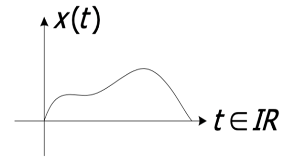
Figure 1 - One-dimensional signal (one argument and one output)

Discrete-time signal $x[n]$ or digital:
A discrete signal has discrete argument(s):

\[ x[n] : \mathbb{N} \to \mathbb{Z} \]

Or, in general:

\[ x : \mathbb{N}^m \to \mathbb{Z}^n \]

import numpy as np
import matplotlib.pyplot as plt

# Discrete signal function: x[n] = 2^n
n_values = np.arange(-5, 6)  # From n = -5 to n = 5
x_values = [2.0**n for n in n_values]

# Plot the discrete signal
plt.stem(n_values, x_values)
plt.title("Discrete Signal: $x[n] = 2^n$")
plt.xlabel("n")
plt.ylabel("$x[n]$")
plt.grid(True)
plt.show()

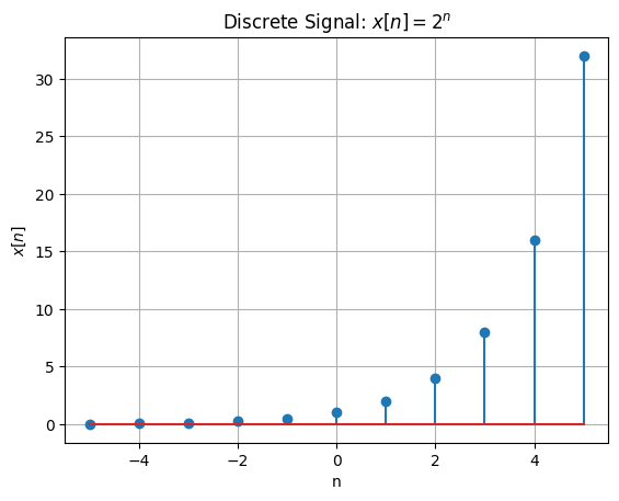
../_images/bddc1768543228d6154a3c024e6b24adf999f225245fa58db8842ff962d8b930.png

Examples of a Signal#

Figure 2 - One-dimensional discrete signal

$n$ and $t$ are independent variables, and $x$ is the dependent variable or function.

In the topic of sampling, we will see that by sampling a continuous-time signal, an approximation of the discrete-time signal can be obtained.

Example of a Discrete Signal#

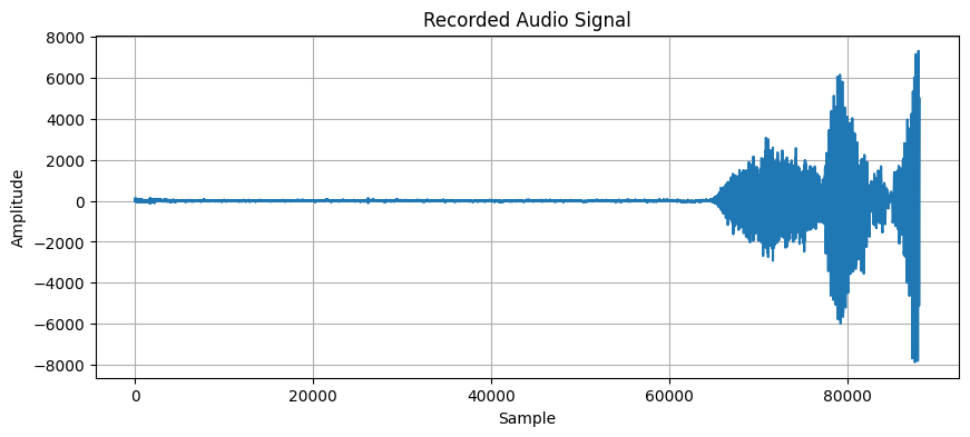
We will capture an audio signal from the microphone using $sounddevice$ in Python and save it to a file, then visualize it.

Python Example: Audio Signal Capture and Plotting#

Figure 3 - Audio Signal Output

import numpy as np
import matplotlib.pyplot as plt
import scipy.io.wavfile as wav

sample_rate, data = wav.read('mySpeech.wav')

# Save the recorded audio to a file

# Plot the audio signal
plt.figure(figsize=(10, 4))
plt.plot(data)
plt.title('Recorded Audio Signal')
plt.xlabel('Sample')
plt.ylabel('Amplitude')
plt.grid()
plt.show()

../_images/f1602a7ef47bcd638bdf9a70dead3f4383d34382e107dbe3ba1023c9dd1b9b39.png

Even and Odd Signals#

Classification Based on Symmetry#

Even Signal#

A signal is even if:

For continuous signals:

\[ x(t) = x(-t) \]

For discrete signals:

\[ x[n] = x[-n] \]

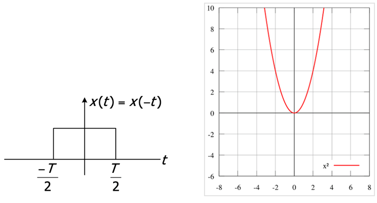
In other words, even functions are symmetric with respect to the y-axis.

Odd Signal#

A signal is odd if:

For continuous signals:

\[ x(t) = -x(-t) \]

For discrete signals:

\[ x[n] = -x[-n] \]

In other words, odd signals are symmetric with respect to the origin.

Examples#

cos(t) is an even signal.
sin(t) is an odd signal.

Properties#

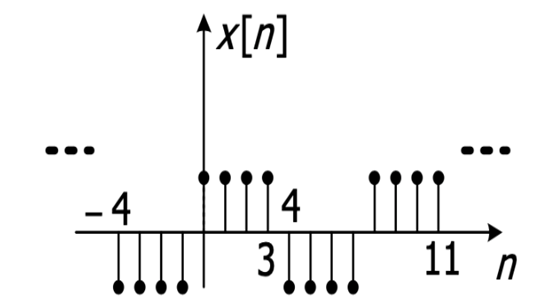
A discrete odd signal must have a value of zero at the origin.

Decomposition#

Any arbitrary signal can be written as the sum of an even and an odd signal:
$$ x(t) = \text{Even}(x(t)) + \text{Odd}(x(t)) $$

Where:

\[ \text{Even}(x(t)) = \frac{1}{2}(x(t) + x(-t)) \]

\[ \text{Odd}(x(t)) = \frac{1}{2}(x(t) - x(-t)) \]

Odd signal odd_Signal_1

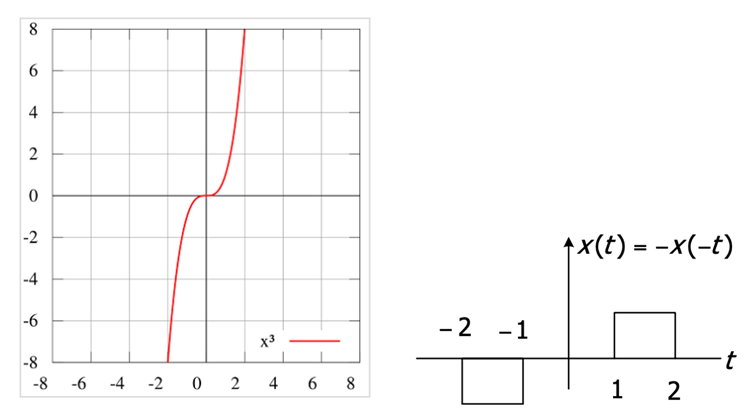
Even Signal Even_Signal_1

Alternating Signals#

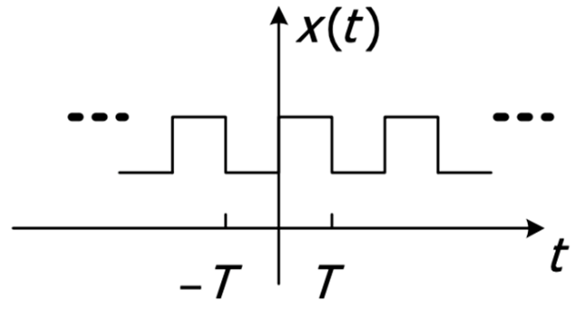
A signal is periodic or alternating if it satisfies the equation

\[ f(t) = f(t + T) \]

where $ T $ is the fundamental period. However, a non-periodic signal does not repeat. An example of a periodic signal is any sinusoidal signal, such as $ \cos(t) $, while an example of a non-periodic signal is a unit impulse.

For continuous signals:

\[ x(t) = x(t + T) = x(t + KT), \quad \omega_0 = \frac{2\pi f}{2\pi/T} \]

For discrete signals:

\[ x[n] = x[n + N] = x[n + KN], \quad \Omega_0 = \frac{2\pi f}{2\pi/T} \]

If $ T $ and $ N $ are periods, multiples such as 2 and 3 times the period are also periods. The smallest period is the fundamental period (T for continuous and N for discrete), and the frequency defined by the smallest period is the fundamental frequency. The period of a continuous-time signal must be positive, while the period of a discrete-time signal must be both positive and integer.

Periodic Signal _Discrete

Periodic Signal _Continious

Operations on Signals#

Signals can be constructed from other signals. In fact, many signals can be defined as combinations of smaller and more fundamental signals. Basic operations on signals fall into two main types: domain operations and time operations.

Domain Operations#

Domain operations on signals affect the amplitude and follow basic mathematical operations, namely addition and multiplication. Adding two signals results in their amplitudes being summed at each point in time. Therefore, adding two signals $ x_0 $ and $ x_1 $ results in a signal $ x_2 $, meaning that at each time, the amplitude of $ x_2 $ is the sum of the amplitudes of $ x_0 $ and $ x_1 $.

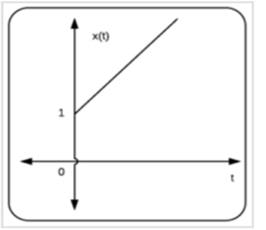
Example: Adding a unit step function to a unit ramp function results in a signal where negative values are zeroed.

Unit_Ramp_1

Time Operations#

We can alter the time of a signal by shifting, scaling, or reversing it.

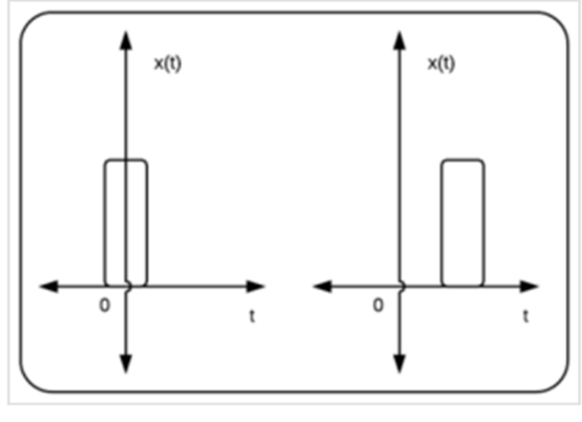
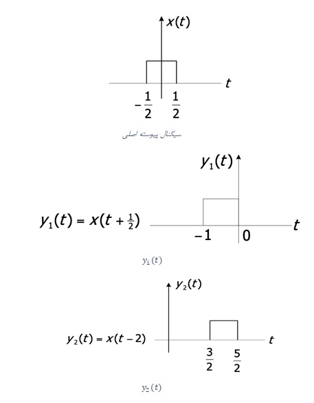
Time shift for continuous signals:

\[ y(t) = x(t - t_0) \]

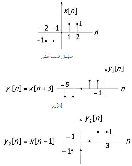
Time shift for discrete signals:

\[ y[n] = x[n - n_0] \]

Right shift: If $ t_0 > 0 $, $ x(t) $ is shifted $ t_0 $ units to the right to get $ y(t) $.
Left shift: If $ t_0 < 0 $, $ x(t) $ is shifted $ t_0 $ units to the left to get $ y(t) $.

If $ t_0 > 0 $, the signal $ x(t - t_0) $ is delayed compared to $ x(t) $, and if $ t_0 < 0 $, the signal $ x(t - t_0) $ is advanced compared to $ x(t) $.

Shift_Right_1

Shift_Discrete

ShiftAnalog_1

Reversal#

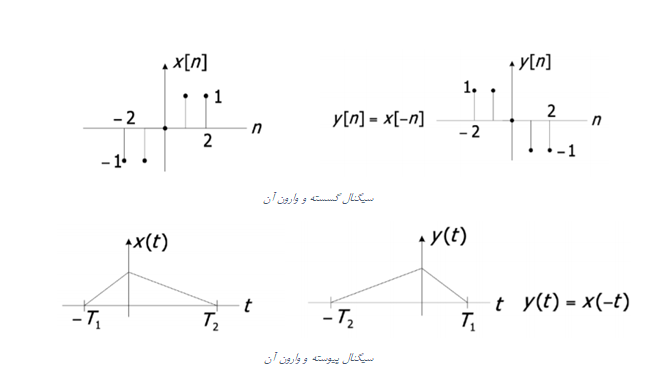
Reversal is an operation where a signal $ f(t) $ is transformed into $ f(-t) $.

For continuous signals:

\[ y(t) = x(-t) \]

For discrete signals:

\[ y[n] = x[-n] \]

Reverse_1

Time Scaling#

Information of a signal can be compressed or expanded in the time domain. For the signal $ x(t) $:

If $ a > 1 $, $ x(at) $ compresses the signal in time.
If $ 0 < a < 1 $, $ x(at) $ expands the signal in time.

If $ a < 0 $, time reversal should be applied after scaling.

Signal Energy Calculation#

Energy of a signal, as one of the transformations (or features of the signal), is discussed in the discrete domain since it is more practical for students.

For example, consider the signal:

\[ x(n) = [1, 2, 3, -1, 2, 5] \]

The energy of the signal is:

\[ \sum x^2(n) = 1^2 + 2^2 + 3^2 + (-1)^2 + 2^2 + 5^2 = 44 \]

In continuous signals, energy is calculated using:

\[ E = \int_{-\infty}^{+\infty} |x(t)|^2 \, dt \]

For discrete signals:

\[ p = \lim_{N \to \infty} \frac{1}{2N+1} \sum_{n=-\infty}^{+\infty} |x[n]|^2 \]

For continuous signals:

\[ p = \lim_{T \to \infty} \frac{1}{2T} \int_{-T}^{+T} |x(t)|^2 \, dt \]

The average power of a signal is known as the signal’s energy if and only if it is bounded.

Energy of Audio Signal#

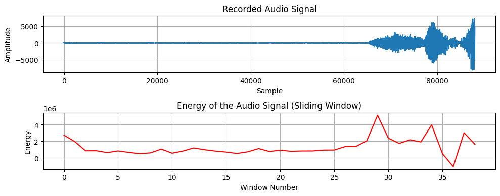
The total energy of a signal, such as audio signals, is not typically calculated over a large time span because the signal’s statistics change over time. Instead, energy is calculated in small windows (i.e., over a small number of data points in a specific part of the time domain). Given the sampling rate of 44,100 Hz (meaning 44,100 samples per second), 44,100 divided by 50 is considered as the frame size. The energy for each of these frames is then calculated as described.

Homework: Segmentation of the Audio Signal by energey#

The discrete signal is shown in the figure. These are discrete signals, meaning their domain (the signal argument) is discrete, while the signal values themselves are continuous but quantized. In exercises and textbooks, the discrete domain is represented by bars, and the origin of time is marked with an underline.

Film 2: Calculation of Digital Signal Energy and Its Application#

import numpy as np
import matplotlib.pyplot as plt
import scipy.io.wavfile as wav

# Step 1: Read the audio file
sample_rate, data = wav.read('mySpeech.wav')

# Step 2: Define the sliding window size (5% of the sample rate)
window_size = int(0.05 * sample_rate)  # 5% of the sample rate

# Step 3: Initialize an array to store the energy values
energy_values = []

# Step 4: Calculate energy using a sliding window approach
for i in range(0, len(data) - window_size, window_size):  # Sliding through the data
    window = data[i:i + window_size]  # Extract the window of samples
    energy = np.sum(window**2)  # Compute the energy (sum of squared values)
    energy_values.append(energy)

# Step 5: Plot the audio signal
plt.figure(figsize=(10, 4))
plt.subplot(2, 1, 1)
plt.plot(data)
plt.title('Recorded Audio Signal')
plt.xlabel('Sample')
plt.ylabel('Amplitude')
plt.grid()

# Step 6: Plot the energy values
plt.subplot(2, 1, 2)
plt.plot(np.arange(len(energy_values)), energy_values, color='r')
plt.title('Energy of the Audio Signal (Sliding Window)')
plt.xlabel('Window Number')
plt.ylabel('Energy')
plt.grid()

# Display the plots
plt.tight_layout()
plt.show()

../_images/33c1d44c25c99d15e0a740e4fd23df81ec4d3997b5dfdf42eaf500277794eb73.png

Application of Energy#

Signal energy is a valuable tool for identifying periods of silence within an audio signal, which plays a crucial role in various signal processing tasks, such as phoneme segmentation and speech recognition. By analyzing the energy levels of the signal, regions of silence or low activity can be distinguished from regions of speech or sound. This is particularly useful in scenarios where speech needs to be separated from background noise or where efficient encoding is required for storage or transmission. For example, the segmentation of a signal based on its energy is illustrated in Figure 20, where distinct segments of the signal are identified and separated according to their energy characteristics.

A widely used method for such tasks is Voice Activity Detection (VAD). VAD is a fundamental technique in speech processing, enabling the detection of human speech within an audio stream. It is commonly employed in speech compression, noise reduction, and automatic speech recognition (ASR) systems. VAD works by analyzing segments of the signal and determining whether each segment contains speech or non-speech (such as silence or noise).

By segmenting the signal into smaller portions, VAD can significantly reduce the size of the audio data by only preserving the sections that contain speech. This is particularly useful in telecommunication and storage systems, where bandwidth and storage space are often limited. VAD helps in improving efficiency by minimizing the amount of data required to represent a speech signal while maintaining the intelligibility and quality of the spoken content.

In addition to reducing storage requirements, VAD plays a key role in improving the performance of speech recognition systems by focusing on relevant portions of the signal, thereby reducing the processing load and increasing accuracy.

Signal Definition

Contents

Signal Definition#