Decomposition#
Discrete Decomposition#
Another example of decomposition on a discrete signal:
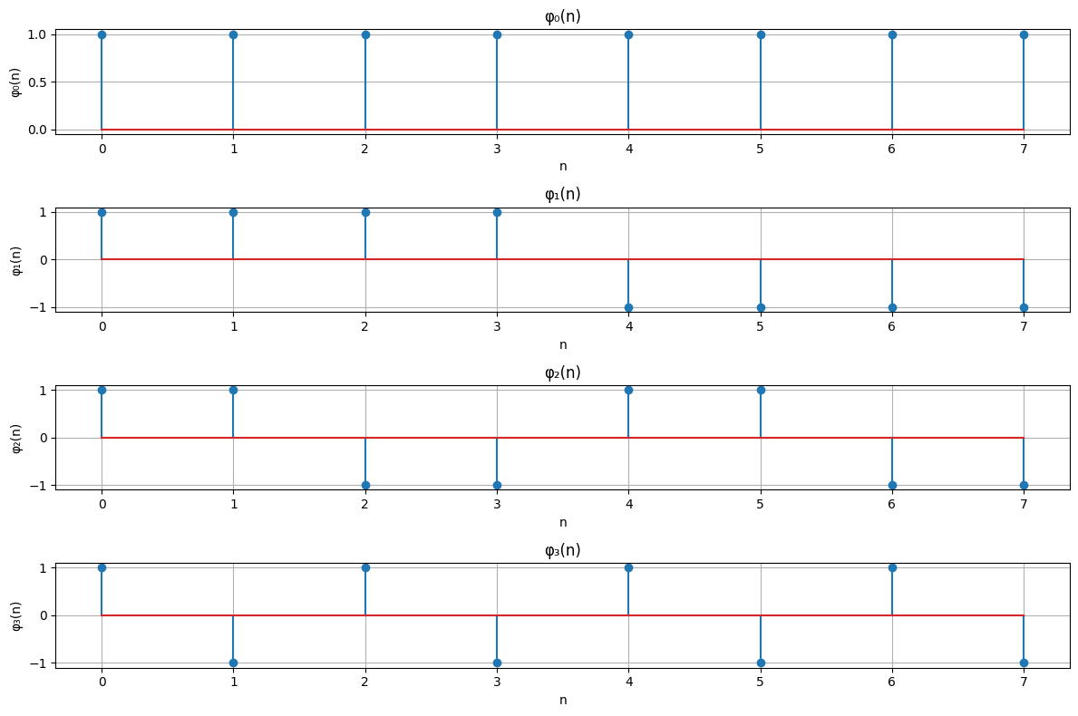
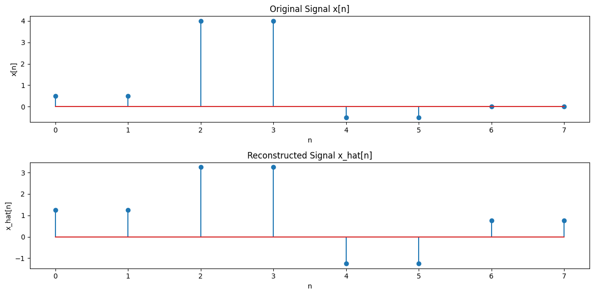
where the basis functions are shown in Figure 1, and the signal is depicted in Figure 2.
To introduce an orthogonal set of basis functions \(\phi_k(n)\) for \(k = 1\) to \(4\) based on your provided definition, let’s define each \(\phi_k(n)\) explicitly. Here, \(\phi_0(n)\) is given, and we will extend the pattern for \(\phi_1(n)\) through \(\phi_3(n)\).
Basis Functions#
\(\phi_0(n)\) $\( \phi_0(n) = \begin{cases} 1 & \text{for } n = 0, 1, 2, 3, 4, 5, 6, 7 \\ 0 & \text{otherwise} \end{cases} \)\( For \)n = 0\( to \)7\(, \)\phi_0(n) = 1$.
\(\phi_1(n)\) $\( \phi_1(n) = \begin{cases} 1 & \text{for } n = 0, 1, 2, 3 \\ -1 & \text{for } n = 4, 5, 6, 7 \\ 0 & \text{otherwise} \end{cases} \)\( For \)n = 0\( to \)3\(, \)\phi_1(n) = 1\(, and for \)n = 4\( to \)7\(, \)\phi_1(n) = -1$.
\(\phi_2(n)\) To generate an orthogonal basis function, we use a pattern of changing signs more frequently. For \(k = 2\), we divide the range into 4 intervals: $\( \phi_2(n) = \begin{cases} 1 & \text{for } n = 0, 1 \\ -1 & \text{for } n = 2, 3 \\ 1 & \text{for } n = 4, 5 \\ -1 & \text{for } n = 6, 7 \\ 0 & \text{otherwise} \end{cases} \)$
\(\phi_3(n)\) We continue to follow the pattern of changing signs more frequently, creating a higher frequency basis function:
\[\begin{split} \phi_3(n) = \begin{cases} 1 & \text{for } n = 0 \\ -1 & \text{for } n = 1 \\ 1 & \text{for } n = 2 \\ -1 & \text{for } n = 3 \\ 1 & \text{for } n = 4 \\ -1 & \text{for } n = 5 \\ 1 & \text{for } n = 6 \\ -1 & \text{for } n = 7 \\ 0 & \text{otherwise} \end{cases} \end{split}\]
Summary#
\(\phi_0(n)\) is a constant function over the entire range.
\(\phi_1(n)\) alternates between 1 and -1 over the range.
\(\phi_2(n)\) alternates signs in blocks.
\(\phi_3(n)\) alternates signs more frequently within the range.
These functions can form an orthogonal set when their inner products are computed over the specified interval. The functions are designed to be orthogonal to each other by construction, typically achieved by ensuring that the integral of their product over the range is zero for \(k \neq l\).
import numpy as np
import matplotlib.pyplot as plt

# Define the basis functions
def phi_0(n):
    return np.ones_like(n)

def phi_1(n):
    return np.where(n < 4, 1, -1)

def phi_2(n):
    return np.where((n % 4) < 2, 1, -1)

def phi_3(n):
    return np.where(n % 2 == 0, 1, -1)

# Define the range of n
n = np.arange(8)

# Plot the basis functions
plt.figure(figsize=(12, 8))

# Plot phi_0
plt.subplot(4, 1, 1)
plt.stem(n, phi_0(n))
plt.title('φ₀(n)')
plt.xlabel('n')
plt.ylabel('φ₀(n)')
plt.grid(True)

# Plot phi_1
plt.subplot(4, 1, 2)
plt.stem(n, phi_1(n))
plt.title('φ₁(n)')
plt.xlabel('n')
plt.ylabel('φ₁(n)')
plt.grid(True)

# Plot phi_2
plt.subplot(4, 1, 3)
plt.stem(n, phi_2(n))
plt.title('φ₂(n)')
plt.xlabel('n')
plt.ylabel('φ₂(n)')
plt.grid(True)

# Plot phi_3
plt.subplot(4, 1, 4)
plt.stem(n, phi_3(n))
plt.title('φ₃(n)')
plt.xlabel('n')
plt.ylabel('φ₃(n)')
plt.grid(True)

plt.tight_layout()
plt.show()
Verify Orthogonality#
To check if the set \(\psi\) including \(\phi_0\), \(\phi_1\), and \(\phi_2\) is orthogonal, you need to verify if the inner products of each pair of basis functions are zero.
Compute Inner Products
To check if \(\phi_0\), \(\phi_1\), and \(\phi_2\) are orthogonal, you need to compute the inner products between each pair:
\(\langle \phi_0, \phi_1 \rangle\)
\(\langle \phi_0, \phi_2 \rangle\)
\(\langle \phi_1, \phi_2 \rangle\)
The inner product is defined as:
where \(i\) and \(j\) are indices of the basis functions.
Check Each Pair
For each pair of basis functions, you should compute:
\(\langle \phi_0, \phi_1 \rangle = \sum_{n \in \mathbb{Z}} \phi_0(n) \phi_1(n)\)
\(\langle \phi_0, \phi_2 \rangle = \sum_{n \in \mathbb{Z}} \phi_0(n) \phi_2(n)\)
\(\langle \phi_1, \phi_2 \rangle = \sum_{n \in \mathbb{Z}} \phi_1(n) \phi_2(n)\)
If all these inner products are zero, then \(\phi_0\), \(\phi_1\), and \(\phi_2\) are orthogonal.
Compute Energy
The energy of each function is given by the inner product of the function with itself:
where \(i\) denotes the index of the basis function. Compute this for each function \(\phi_0\), \(\phi_1\), and \(\phi_2\).
Compute ceoficients#
To decompose the signal \( x[n] = [\frac{1}{2}, \frac{1}{2}, 4, 4, -\frac{1}{2}, -\frac{1}{2}] \) using the orthogonal basis functions \(\phi_0, \phi_1, \phi_2, \phi_3\), follow these steps:
1. Compute the Energy of Each Basis Function \( E_{\phi_k} \)#
The energy \( E_{\phi_k} \) of each basis function \(\phi_k\) is given by: $\( E_{\phi_k} = \sum_{n} \phi_k(n)^2 \)$
Basis Functions:
\(\phi_0(n)\): 1 for all \( n \)
\(\phi_1(n)\): 1 for \( n = 0, 1, 2, 3 \) and -1 for \( n = 4, 5, 6, 7 \)
\(\phi_2(n)\): 1 for \( n \% 4 = 0, 1 \) and -1 for \( n \% 4 = 2, 3 \)
\(\phi_3(n)\): 1 for even \( n \) and -1 for odd \( n \)
Let’s compute \( E_{\phi_k} \) for each function:
For \(\phi_0(n)\):
For \(\phi_1(n)\):
For \(\phi_2(n)\):
For \(\phi_3(n)\): $\( E_{\phi_3} = \sum_{n=0}^{7} \phi_3(n)^2 = 4 + 4 = 8 \)$
Compute the Coefficients \( a_k \)#
The coefficient \( a_k \) for each basis function \(\phi_k\) is computed using:
where \(\langle x(n), \phi_k(n) \rangle\) is the inner product:
Computing \( a_k \):
For \( \phi_0(n) \):
For \( \phi_1(n) \):
For \( \phi_2(n) \):
For \( \phi_3(n) \):
Compute the Approximation \( \hat{x}[n] \)#
Combine the basis functions to approximate \( x[n] \):
For \( k = 0 \): \( a_0 = 1 \)
For \( k = 1 \): \( a_1 = 1.25 \)
For \( k = 2 \): \( a_2 = -1 \)
For \( k = 3 \): \( a_3 = 0 \)
Using the basis functions:
Comparison#
To compare \(\hat{x}[n]\) with \(x[n]\), plot or print the values of \(\hat{x}[n]\) and \(x[n]\).
Values of \(x[n]\): $\( x[n] = [\frac{1}{2}, \frac{1}{2}, 4, 4, -\frac{1}{2}, -\frac{1}{2}, 0, 0] \)$
Values of \(\hat{x}[n]\) (approximation): Calculate \(\hat{x}[n]\) using the defined basis functions and coefficients.
This process will give you an approximate representation of \(x[n]\) using the orthogonal basis functions.
import numpy as np
import matplotlib.pyplot as plt

# Define basis functions
def phi_0(n):
    return np.ones_like(n)

def phi_1(n):
    return np.where(n < 4, 1, -1)

def phi_2(n):
    a=[1, 1, -1, -1, 1, 1, -1, -1]
    return np.array(a)

def phi_3(n):
    return np.array([1 ,-1, 1, -1, 1, -1, 1, -1])

# Mapping for basis functions
def basis_functions(n, k):
    """Return the basis function φ_k(n) for index k."""
    if k == 0:
        return phi_0(n)
    elif k == 1:
        return phi_1(n)
    elif k == 2:
        return phi_2(n)
    elif k == 3:
        return phi_3(n)
    else:
        # Extend this mapping for more basis functions if needed
        raise ValueError(f"Basis function φ_{k}(n) not defined.")

def calculate_alpha(x, n, k):
    """Calculate the coefficient α_k for basis function φ_k(n)."""
    phi_k_n = basis_functions(n, k)
    E_phi_k = np.sum(phi_k_n**2)   # Normalize E_phi_k
    return np.sum(x * phi_k_n) / E_phi_k

def reconstruct_signal(n, coefficients, max_basis):
    """Reconstruct the signal x_hat[n] using the coefficients and basis functions."""
    x_hat = np.zeros_like(n, dtype=float)
    for k in range(max_basis + 1):  # +1 to include K
        phi_k_n = basis_functions(n, k)
        x_hat += coefficients[k] * phi_k_n
    return x_hat

# Define the indices and original signal
n = np.arange(8)
x = np.array([1/2, 1/2, 4, 4, -1/2, -1/2, 0, 0])

# Specify the number of basis functions (K)
K = 3  # Change this value to include more basis functions if defined

# Calculate coefficients
coefficients = [calculate_alpha(x, n, k) for k in range(K + 1)]

# Reconstruct the signal
x_hat = reconstruct_signal(n, coefficients, K)

# Plot original and reconstructed signals
plt.figure(figsize=(12, 6))

plt.subplot(2, 1, 1)
plt.stem(n, x)
plt.title('Original Signal x[n]')
plt.xlabel('n')
plt.ylabel('x[n]')

plt.subplot(2, 1, 2)
plt.stem(n, x_hat)
plt.title('Reconstructed Signal x_hat[n]')
plt.xlabel('n')
plt.ylabel('x_hat[n]')

plt.tight_layout()
plt.show()

# Print coefficients
print("Coefficients:")
for k in range(K + 1):
    print(f"α_{k} = {coefficients[k]:.3f}")
Coefficients:
α_0 = 1.000
α_1 = 1.250
α_2 = -1.000
α_3 = 0.000
Homework: Decompose with Haar#
Write a complete implementation based on the code discussed above. Ensure that your code is fully functional and includes all necessary components to achieve the desired results. Be thorough in your documentation and include comments where necessary to explain your logic and methodology.
Fourier Decomposition#
The final example of decomposition is presented to conclude the introduction of the topic in the lesson. We have become sufficiently familiar with the decomposition and will now move on to discussing systems.
Example: The following set is introduced: $\( \psi = \{ e^{jk\omega_0 t} ; k \in \mathbb{Z} \} \)$
(Equation 4)
The first step in the decomposition is to check the orthogonality of the given set. If it is not orthogonal, it must be solved by another method, but there is no need to solve it this way.
(Equation 5)
If Equation 5 equals zero, the set will be orthogonal.
(Equation 6)
We know that the integrals of sine and cosine over their period are zero. Thus, for \(k - l\), it is also zero because \(k\) is not equal to \(l\) and \(k - l\) does not become zero. Hence, Equation 6 equals zero, so the set \(\psi\) is orthogonal.
Now, we calculate Equation 5 for \(k = l\):
Thus, in general, we have:
Therefore, \(\psi\) is an orthogonal set.
In the second step, the coefficients \(\alpha\) must be calculated, which are obtained from the following relation:
(Equation 7)
Substituting into Equation 7, we have:
(Equation 8)
import sympy
i2pi = sympy.I*2*sympy.pi # i2pi is shorthand for 2πi (imaginary part)
exp = sympy.exp # The exponential function from sympy
def S(N):
    return sum(c(n)*exp(i2pi*n*t/P) for n in range(-N, N+1)).expand(complex=True).simplify()
def c(n):
    return (sympy.integrate(
               f(t)*exp((-i2pi * n * t)/P),
               (t, t0, t0 + P))/P)

#  These functions work quite well for a periodic sawtooth function:

a = sympy.Symbol('a', positive=True)
def f(t):
    return t

P = 20  # Period of the sawtooth wave
t0 = -10  # Starting point of the period
t = sympy.Symbol('t', real=True)  # Symbolic variable for time
N = 4  # Number of Fourier terms (harmonics)

analytic_approx = S(N).expand()
analytic_approx
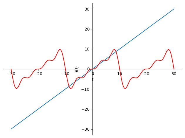
Notice Fourier series do over periodic signals#
Notice that the function we defined was just \( y=t \) , but Fourier series always approximates periodic signals. We can see the bit we approximated repeating if we plot over a larger interval
interval = (t, t0 - P, t0 + 2 * P)  # Define the interval for plotting
p1 = sympy.plot(f(t), interval, show=False)  # Plot the original sawtooth function
p2 = sympy.plot(analytic_approx, interval, show=False)  # Plot the Fourier approximation

p2[0].line_color = 'red'  # Set Fourier series plot color to red
p1.extend(p2)  # Combine the original and Fourier series plots
p1.show()  # Display the combined plot
from sympy import fourier_series, pi
from sympy.abc import x


f = x**2  # Define the function f(x) = x^2

N = 4  # Number of Fourier terms (harmonics)
s = fourier_series(f, (x, -pi, pi))  # Compute the Fourier series of f over [-pi, pi]
s1 = s.truncate(n=N)  # Truncate the series to 3 terms (n=3)
s1
import sympy
from sympy import fourier_series, pi
from sympy.plotting import plot

# Define symbolic variable for time
t = sympy.Symbol('t', real=True)

# Define the periodic quadratic function f(t) = t^2
def f(t):
    return t**2

# Define parameters
P = 8  # Period of the wave
t0 = -2  # Starting point of the period

# Compute the Fourier series for f(t) = t^2 over the interval [-P/2, P/2]
N = 20  # Number of Fourier terms (harmonics)
s = fourier_series(f(t), (t, t0, t0 + P))  # Compute Fourier series
s1 = s.truncate(n=N)  # Truncate to the first N terms (N harmonics)

# Define the interval for plotting
interval = (t, t0 - P, t0 + 2 * P)

# Plot the original function f(t) = t^2
p1 = plot(f(t), interval, show=False, label='Original function')

# Plot the truncated Fourier series approximation
p2 = plot(s1, interval, show=False, line_color='red', label=f'Fourier Series Approx (N={N})')

# Combine the two plots
p1.extend(p2)

# Set colors for better visualization
p1[0].line_color = 'blue'  # Set the color of the original function
p1[1].line_color = 'red'   # Set the color of the Fourier approximation

# Show the combined plot
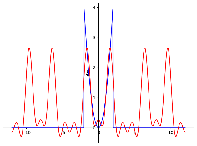
p1.show()
import sympy
from sympy import fourier_series, pi
from sympy.plotting import plot

# Define symbolic variable for time
t = sympy.Symbol('t', real=True)

# Define the periodic piecewise quadratic function f(t) = t^2 for -2 <= t <= 2, and 0 elsewhere
def f(t):
    return sympy.Piecewise((t**2, (t >= -2) & (t <= 2)), (0, True))

# Define parameters
P = 8  # Period of the wave
t0 = -P / 2  # Starting point of the period (centered around 0)

# Compute the Fourier series for f(t) over the interval [-P/2, P/2]
N = 6  # Number of Fourier terms (harmonics)
s = fourier_series(f(t), (t, t0, t0 + P))  # Compute Fourier series over [-P/2, P/2]
s1 = s.truncate(n=N)  # Truncate to the first N terms (N harmonics)

# Define the interval for plotting
interval = (t, t0 - P, t0 + 2 * P)  # Extend the plot over two periods

# Plot the original function f(t)
p1 = plot(f(t), interval, show=False, label='Original function')

# Plot the truncated Fourier series approximation
p2 = plot(s1, interval, show=False, line_color='red', label=f'Fourier Series Approx (N={N})')

# Combine the two plots
p1.extend(p2)

# Set colors for better visualization
p1[0].line_color = 'blue'  # Set the color of the original function
p1[1].line_color = 'red'   # Set the color of the Fourier approximation

# Show the combined plot
p1.show()
Signal Decomposition#
This session is dedicated to decomposing a signal into basic signals. In other words, the signal \( x(t) \) is written as a linear combination of the basic signals: $\( x(t) = \sum a_k \phi_k(t) \)\( The basic signals are chosen from the set \) \psi \(. The set \) \psi \( is an orthogonal set: \)\( \psi = \{ \phi_k(t) ; k \in \mathbb{Z} \} \)$
If two signals \( w(t) \) and \( v(t) \) are non-periodic signals, the inner product of the two signals is defined as: $\( \langle v(t), w(t) \rangle = \lim_{T \to \infty} \int_{-T/2}^{T/2} v(t) w^*(t) \, dt \)$
If two signals \( w(t) \) and \( v(t) \) are periodic with a common period \( T_0 \), the inner product of the two signals is defined as: $\( \langle v(t), w(t) \rangle = \lim_{T_0 \to \infty} \frac{1}{T_0} \int_{-T_0/2}^{T_0/2} v(t) w^*(t) \, dt \)$
For orthogonal signals, the inner product equals zero. Therefore, they are orthogonal if: $\( \langle v(t), w(t) \rangle = 0 \)$
Inner product properties#
The orthogonal set is checked using the inner product. The inner product of \( x \) and \( y \), denoted as \( \langle x, y \rangle \), has several properties as follows:
\( \langle ax, y \rangle = a \langle x, y \rangle \)
\( \langle x + y, z \rangle = \langle x, z \rangle + \langle y, z \rangle \)
\( \langle x, y \rangle = \overline{\langle y, x \rangle} \)
\( \langle x, x \rangle > 0 \quad \text{if} \quad x \neq 0 \)
\( \langle x, x \rangle \geq 0 \)
The inner product of linear combinations of \( x_n \) and \( y \) can be expanded as follows: $\( \langle \sum a_n x_n , y \rangle = \sum a_n \langle x_n, y \rangle \)$
For example: $\( \langle \sum a_k \phi_k(t) , g(t) \rangle = \langle a_1 \phi_1(t) + \dots + a_n \phi_n(t), g(t) \rangle = \langle a_1 \phi_1(t), g(t) \rangle + \dots + \langle a_n \phi_n(t), g(t) \rangle = \sum a_k \langle \phi_k(t), g(t) \rangle \)$
Commutativity property of the inner product of two functions \( x(t) \) and \( y(t) \): $\( \langle x(t), y(t) \rangle = \int x(t) y(t)^* dt = \left( \int x(t)^* y(t) dt \right)^* = \left( \langle y(t), x(t) \rangle \right)^* \)$
Some examples of the inner product of functions: $\( \langle x, x^2 \rangle = \int_0^2 x \cdot x^2 \, dx = \frac{1}{4} \)$
Another example: If \( x(t) \) is given by:
The goal is to find the coefficients \( a \). To find the coefficient \( a_{-1} \), we have:
Since \( \phi \in \psi \) and the set \( \psi \) is orthogonal, if the \( \phi \)‘s are not the same, their inner product equals zero. Therefore, Equation 12 becomes:
Thus, each coefficient can be found as:
