Linear approximation

Author: Reza Farasati

Contact: rezafarasati2004@gmail.com

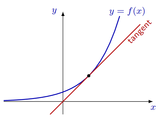
In applications, we may encounter difficulties in finding exact solutions to the problems. Often approximate solutions are acceptable within some tolerance. The simplest approximation of a function is given by a linear function. In this section, we will study how a differentiable function may be approximated by a linear function. We already know that the tangent line goes very close to the graph of the function. The tangent line describes the behavior of the function near the point of tangency better than any other line. It makes sense to use the tangent line as a linear approximation to the graph.

Taylor Series Expansion

For a function \( f(x) \), the Taylor series expansion around a point \( a \) is given by:

\[ f(x) \approx f(a) + f'(a)(x - a) + \frac{f''(a)}{2!}(x - a)^2 + \frac{f'''(a)}{3!}(x - a)^3 + \cdots \]

Maclaurin Series

If the expansion is around \( a = 0 \), it is called the Maclaurin series:

\[ f(x) \approx f(0) + f'(0)x + \frac{f''(0)}{2!}x^2 + \frac{f'''(0)}{3!}x^3 + \cdots \]

Linearization

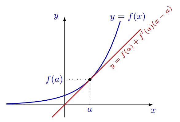
Let \( f \) be a function differentiable at the point \( x = a \) . The equation of the tangent line to the graph of f at the point \( x = a \) is

\( y = f (a) + f'(a)(x − a) \)

Definition

The linearization, or linear approximation, of the function \( f \) near point \( x = a \) is the linear function \( L(x) = f (a) + f'(a)(x − a) \) \( f (x) ≈ L(x) \) near \( x = a \)

Examples of Linearization

Example 1:

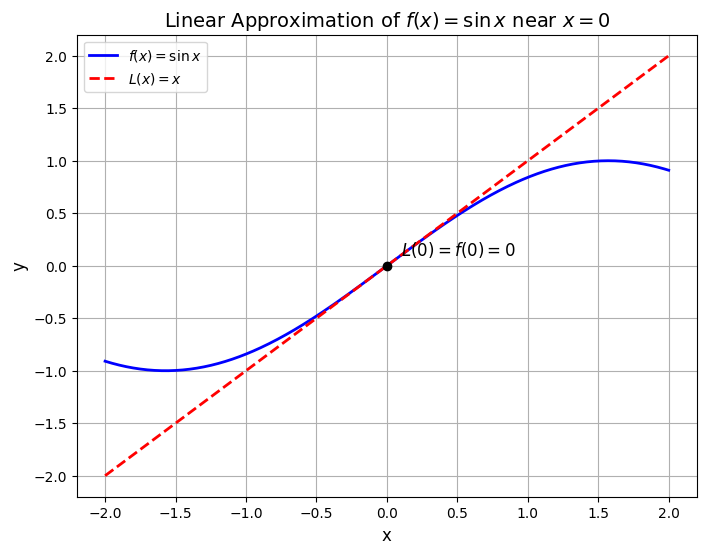
Find the linear approximation to \(f(x) = \sin x\) near \(x = 0\).

The linear approximation is the function:

\[ L(x) = f(a) + f'(a)(x - a) \]

where \(f(x) = \sin x\) and \(a = 0\).

Since

\[ f'(0) = f'(x) \bigg|_{x=0} = \left( \sin x \right)' \bigg|_{x=0} = \cos x \bigg|_{x=0} = \cos 0 = 1 \]

and

\[ f(0) = \sin 0 = 0 \]

we find:

\[ L(x) = 0 + 1 \cdot (x - 0) \quad \Longleftrightarrow \quad L(x) = x \]

The linear function approximating \(f(x) = \sin x\) near \(x = 0\) is \(L(x) = x\).

Here is the code:

import numpy as np
import matplotlib.pyplot as plt

# Define the original function f(x) = sin(x)
def f(x):
    return np.sin(x)

# Define the linear approximation L(x) = x
def L(x):
    return x

# Create an array of x values from -2 to 2 for plotting
x = np.linspace(-2, 2, 400)

# Calculate the corresponding y values for f(x) and L(x)
y_f = f(x)
y_L = L(x)

# Plotting the graph
plt.figure(figsize=(8, 6))
plt.plot(x, y_f, label=r'$f(x) = \sin x$', color='b', linewidth=2)
plt.plot(x, y_L, label=r'$L(x) = x$', color='r', linestyle='--', linewidth=2)

# Highlight the approximation at x = 0
plt.scatter(0, 0, color='black', zorder=5)
plt.text(0.1, 0.1, r'$L(0) = f(0) = 0$', fontsize=12)

# Add labels and title
plt.title(r'Linear Approximation of $f(x) = \sin x$ near $x = 0$', fontsize=14)
plt.xlabel('x', fontsize=12)
plt.ylabel('y', fontsize=12)

# Add a legend
plt.legend(loc='upper left')

# Show grid
plt.grid(True)

# Display the plot
plt.show()

Example 2:

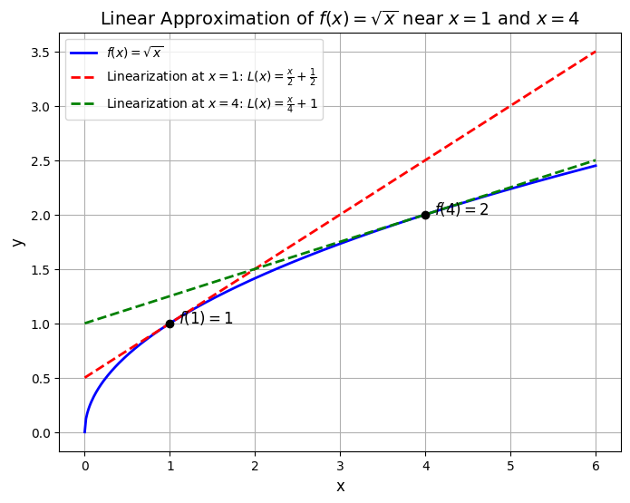
Find the linear approximations to \(f(x) = \sqrt{x}\) near \(x = 1\) and \(x = 4\).

The derivative of \(f(x) = \sqrt{x}\) is:

\[ f'(x) = \frac{1}{2\sqrt{x}} \]

So,

\[ f'(1) = \frac{1}{2}, \quad f'(4) = \frac{1}{2\sqrt{4}} = \frac{1}{4} \]

The linearization near \(x = 1\) is:

\[ L(x) = f(1) + f'(1)(x - 1) \quad \Longleftrightarrow \quad L(x) = 1 + \frac{1}{2}(x - 1) \quad \Longleftrightarrow \quad L(x) = \frac{x}{2} + \frac{1}{2} \]

The linearization near \(x = 4\) is:

\[ L(x) = f(4) + f'(4)(x - 4) \quad \Longleftrightarrow \quad L(x) = 2 + \frac{1}{4}(x - 4) \quad \Longleftrightarrow \quad L(x) = \frac{x}{4} + 1 \]

import numpy as np
import matplotlib.pyplot as plt

# Define the original function f(x) = sqrt(x)
def f(x):
    return np.sqrt(x)

# Define the linear approximations near x = 1 and x = 4
def L1(x):
    return (x / 2) + (1 / 2)

def L4(x):
    return (x / 4) + 1

# Create an array of x values for plotting
x = np.linspace(0, 6, 400)

# Calculate the corresponding y values for f(x), L1(x), and L4(x)
y_f = f(x)
y_L1 = L1(x)
y_L4 = L4(x)

# Plotting the graph
plt.figure(figsize=(8, 6))
plt.plot(x, y_f, label=r'$f(x) = \sqrt{x}$', color='b', linewidth=2)
plt.plot(x, y_L1, label=r'Linearization at $x=1$: $L(x) = \frac{x}{2} + \frac{1}{2}$', color='r', linestyle='--', linewidth=2)
plt.plot(x, y_L4, label=r'Linearization at $x=4$: $L(x) = \frac{x}{4} + 1$', color='g', linestyle='--', linewidth=2)

# Highlight the points at x = 1 and x = 4
plt.scatter(1, f(1), color='black', zorder=5)
plt.scatter(4, f(4), color='black', zorder=5)
plt.text(1.1, f(1), r'$f(1) = 1$', fontsize=12)
plt.text(4.1, f(4), r'$f(4) = 2$', fontsize=12)

# Add labels and title
plt.title(r'Linear Approximation of $f(x) = \sqrt{x}$ near $x = 1$ and $x = 4$', fontsize=14)
plt.xlabel('x', fontsize=12)
plt.ylabel('y', fontsize=12)

# Add a legend
plt.legend(loc='upper left')

# Show grid
plt.grid(True)

# Display the plot
plt.show()

Example 3: Approximate calculations

Use linearization to find an approximate value for \(\frac{1}{1.99}\). Is this approximation an overestimate or an underestimate?

We can easily find the value of \(\frac{1}{2}\), and since \(1.99\) is near \(2\), we may use the linear approximation:

\[ L(x) = f(a) + f'(a)(x - a) \]

for \(f(x) = \frac{1}{x}\) and \(a = 2\).

We calculate the derivative:

\[ f'(x) = \left( \frac{1}{x} \right)' = -\frac{1}{x^2} \]

At \(x = 2\):

\[ f'(2) = -\frac{1}{4} \]

Since \(f(2) = \frac{1}{2}\), we have:

\[ L(x) = \frac{1}{2} - \frac{1}{4}(x - 2) \]

To approximate \(\frac{1}{1.99}\):

\[ \frac{1}{1.99} = f(1.99) \approx L(1.99) = \frac{1}{2} - \frac{1}{4}(1.99 - 2) \]

This simplifies to:

\[ L(1.99) = 0.5 + \frac{0.01}{4} = 0.5 + 0.0025 = 0.5025 \]

Conclusion: Overestimate or Underestimate?

Now we have to answer the question:
Is the obtained approximation an overestimate or an underestimate?
That is, is the approximation \(0.5025\) greater than or less than the true value of \(\frac{1}{1.99}\)?

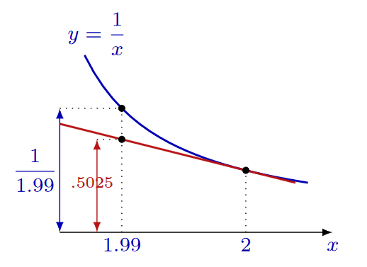
Since the tangent line is below the graph of the function \(f(x) = \frac{1}{x}\) near \(x = 2\), the approximate value, \(0.5025\), is less than the actual value of \(\frac{1}{1.99}\).

Using a calculator:

\[ \frac{1}{1.99} = 0.502512... \]

The linearization gave four correct decimals!

Example 4: Approximation of functions

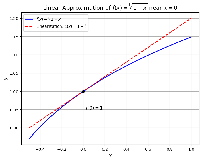
Show that \(\sqrt[5]{1 + x} \approx 1 + \frac{x}{5}\) for small \(x\).

Consider the function \(f(x) = \sqrt[5]{1 + x}\). It is differentiable at \(x = 0\). Therefore, by linearization:

\[ f(x) \approx L(x) = f(0) + f'(0)(x - 0) \]

for \(x\) near \(0\).

We calculate the derivative of \(f(x)\):

\[ f'(x) = \frac{d}{dx} \left( (1 + x)^{\frac{1}{5}} \right) = \frac{1}{5}(1 + x)^{-\frac{4}{5}} \]

At \(x = 0\):

\[ f'(0) = \frac{1}{5} \]

So the linearization near \(x = 0\) is:

\[ f(x) \approx L(x) = f(0) + f'(0)(x - 0) = 1 + \frac{x}{5} \]

as required.

import numpy as np
import matplotlib.pyplot as plt

# Define the original function f(x) = (1 + x)^(1/5)
def f(x):
    return (1 + x)**(1/5)

# Derivative of f(x) at x = 0 is f'(0) = 1/5
def L(x):
    return 1 + (x / 5)

# Create an array of x values for plotting
x = np.linspace(-0.5, 1, 400)

# Calculate the corresponding y values for f(x) and L(x)
y_f = f(x)
y_L = L(x)

# Plotting the graph
plt.figure(figsize=(8, 6))
plt.plot(x, y_f, label=r'$f(x) = \sqrt[5]{1+x}$', color='b', linewidth=2)
plt.plot(x, y_L, label=r'Linearization: $L(x) = 1 + \frac{x}{5}$', color='r', linestyle='--', linewidth=2)

# Highlight the point at x = 0
plt.scatter(0, f(0), color='black', zorder=5)
plt.text(0.02, f(0) - 0.05, r'$f(0) = 1$', fontsize=12)

# Add labels and title
plt.xlabel('x', fontsize=12)
plt.ylabel('y', fontsize=12)
plt.title(r'Linear Approximation of $f(x) = \sqrt[5]{1 + x}$ near $x = 0$', fontsize=14)

# Add a legend
plt.legend(loc='upper left')

# Show grid
plt.grid(True)

# Display the plot
plt.show()

Tangent Plane Approximation

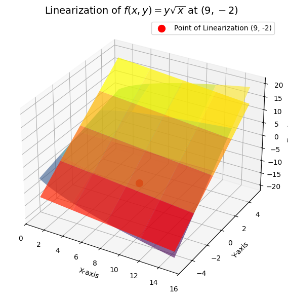
Partial derivatives allow us to approximate functions just like ordinary derivatives do, but with a contribution from each variable. In one-dimensional calculus, we tracked the tangent line to get a linearization of a function. For functions of several variables, we track the tangent plane. The equation of the tangent plane at \((a, b, f(a, b))\) is:

\[ z = f(a, b) + (x - a) f_x(a, b) + (y - b) f_y(a, b) \]

The Linearization of a function \(f(x, y)\) at \((a, b)\) is:

\[ L(x, y) = f(a, b) + (x - a) f_x(a, b) + (y - b) f_y(a, b) \]

This is very similar to the familiar formula for functions of one variable:

\[ L(x) = f(a) + f'(a)(x - a) \]

except that it has an extra term for the second variable. The corresponding formulas for functions of more than two variables are similar, with one term for each variable.

Now, let’s use the linearization \(L(x, y)\) of \(f\) to estimate the change \(\Delta f\) in \(f\) near \((a, b)\):

\[ \Delta f = f(x, y) - f(a, b) \approx L(x, y) - f(a, b) = f_x(a, b) \Delta x + f_y(a, b) \Delta y \]

This is sometimes written using differentials as:

\[ df = f_x(a, b) \, dx + f_y(a, b) \, dy \]

Example 5:

Find the Linearization, \(L(x, y)\), of \(z = f(x, y) = y \sqrt{x}\) at the point \((9, -2)\).

The Linearization of \(f\) at \((a, b)\) is:

\[ L(x, y) = f(a, b) + f_x\big|_{(a, b)}(x - a) + f_y\big|_{(a, b)}(y - b) \]

But when \(f(x, y) = y \sqrt{x}\), we have the partial derivatives:

\[ \frac{\partial f}{\partial x} = \frac{y}{2 \sqrt{x}}, \quad \frac{\partial f}{\partial y} = \sqrt{x} \]

At \((9, -2)\), therefore:

\[ f(9, -2) = -6, \quad f_x\big|_{(9, -2)} = -\frac{1}{3}, \quad f_y\big|_{(9, -2)} = 3 \]

Thus:

\[ L(x, y) = -6 - \frac{1}{3}(x - 9) + 3(y + 2) \]

which after rearrangement becomes:

\[ L(x, y) = 3 - \frac{1}{3}x + 3y \]

import numpy as np
import matplotlib.pyplot as plt
from mpl_toolkits.mplot3d import Axes3D

# Define the function f(x, y) = y * sqrt(x)
def f(x, y):
    return y * np.sqrt(x)

# Define the linearization L(x, y)
def L(x, y):
    return 3 - (1/3) * x + 3 * y

# Generate values for x and y
x = np.linspace(1, 15, 400)
y = np.linspace(-5, 5, 400)
X, Y = np.meshgrid(x, y)

# Compute the values for f(x, y) and the linearization L(x, y)
Z_f = f(X, Y)
Z_L = L(X, Y)

# Plot the function and its linearization (tangent plane)
fig = plt.figure(figsize=(10, 7))
ax = fig.add_subplot(111, projection='3d')

# Plot the surface for f(x, y)
ax.plot_surface(X, Y, Z_f, cmap='viridis', alpha=0.6, rstride=100, cstride=100)

# Plot the surface for the tangent plane L(x, y)
ax.plot_surface(X, Y, Z_L, cmap='autumn', alpha=0.7, rstride=100, cstride=100)

# Plot the point of linearization
ax.scatter(9, -2, f(9, -2), color='red', s=100, label="Point of Linearization (9, -2)")

# Labels and title
ax.set_title("Linearization of $f(x, y) = y \\sqrt{x}$ at $(9, -2)$", fontsize=14)
ax.set_xlabel('X-axis')
ax.set_ylabel('Y-axis')
ax.set_zlabel('Z-axis')

# Show the plot
plt.legend()
plt.show()

References:

1. https://web.ma.utexas.edu/users/m408m/Display14-4.shtml

2. https://www.math.stonybrook.edu/Videos/MAT131Online/Handouts/Lecture-16-Handout.pdf